SUMMARIZE DIALOGUES

Summarizing Client calls

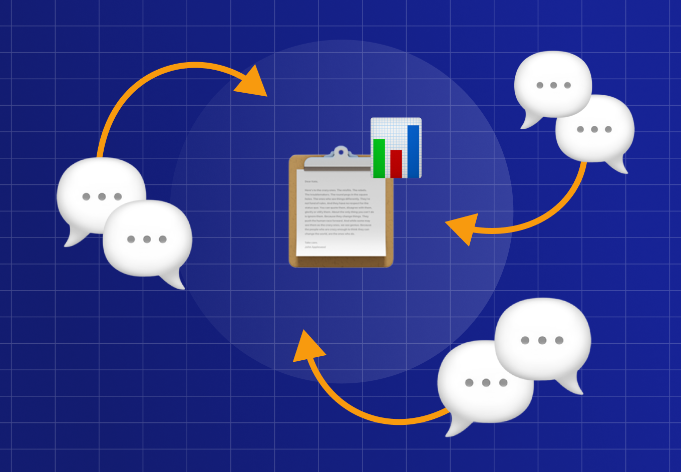
Dialogue summary is an easy way to analyze previous conversations with customers. It allows you to have a good grasp of the discussion without the need to read lengthy transcripts. Every summary analysis provides mentioned topics, keywords, intents, sentiment and more.

The rest of the article is available on the link below:

https://colab.research.google.com/drive/1pMk7JcKVrYT6YTwThMqGGYuFL9Bpc6Xl?usp=sharing#scrollTo=L3nE3kKnhDW9

(NOTICE) In order to be able to use the notebook and send requests to our services, you have to upload a 'credentials.ini’ file to the runtime workspace (the main directory, next to sample_data folder). You can obtain one by getting in touch over at https://voicelab.ai/contact.

Author: Alicja Golisowicz, Patrycja Biryło

Annotate your data

Annotate your data

When developing an NLP solution it is often problematic to transfer the model to a new domain. The issue might be a lack of properly annotated dataset or one that is not big enough to provide full domain knowledge, even though you have a lot of audio recordings available. Annotating additional, large volumes of your data might be very costly and cost-inefficient, especially when dealing with multiple languages, since you’ll need separate teams for each one. However, you can make use of that data in an unsupervised learning manner – it is proven to greatly increase model comprehension on examples similar to those from pre-training phase. The recordings simply need to be properly formatted.

The rest of the article is available on the link below: https://colab.research.google.com/drive/1Uw7yV1iA2oBmnVPyRIQHmJXoSiER_yUG?usp=sharing

(NOTICE) In order to be able to use the notebook and send requests to our services, you have to upload a 'credentials.ini’ file to the runtime workspace (the main directory, next to sample_data folder). You can obtain one by getting in touch over at https://voicelab.ai/contact.

Author: Patryk Neubauer

Why are clients calling?

Discovering clients’ reasons for contact

Adressing customer wants and needs is crucial for prosperous business operations. However, it is not always easy, the amount of contacts every day can get overwhelming and it might be challenging to discover the most common issues. With the help of our Intent Recognition and Reason for Calling module you can quickly reveal the subjects that your clients struggle with the most often. You might also discover problems that you have not been aware of. With such knowledge in hand you can design much more effective FAQ that will take a great burden off of your arms or improve the product/service in ways that you wouldn’t have thought of otherwise. But how to achieve that?

The rest of the article is available on the link below:
https://colab.research.google.com/drive/1g1RLbMeTXuDyFszCjNnp8WM-6DnTP-M4

(NOTICE) In order to be able to use the notebook and send requests to our services, you have to upload a 'credentials.ini’ file to the runtime workspace (the main directory, next to sample_data folder). You can obtain one by getting in touch over at https://voicelab.ai/contact.

Author: Patryk Neubauer

Predicting impactful agent statements

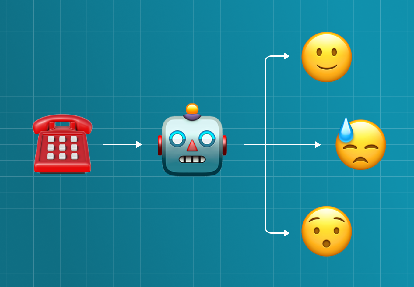
Often it’s hard to know what makes your clients react in one way or another. Some things related to the company or what your agents are saying, might have particularly high impact on your clients – whether it’s negative or positive, it’s useful to know what causes it. Combining our Sentiment Classification and Intent prediction you can find out which agent statements are of high impact to clients.

The rest of the article is available on the link below:

https://colab.research.google.com/drive/1WAmM4T-slDLXhd64-NimaQY0_juZAe9V?usp=sharing

(NOTICE) In order to be able to use the notebook and send requests to our services, you have to upload a 'credentials.ini’ file to the runtime workspace (the main directory, next to sample_data folder). You can obtain one by getting in touch over at https://voicelab.ai/contact.

Author: Filip Żarnecki

VOICELAB – CA API – THE ROOT OF YOUR DATA SCIENCE PROJECT

Getting to know your data

Knowing the data you plan to be working with is probably the most crucial aspect of any data science project. And getting to know a new, huge, unstructured corpus might be a bit of a pain to carry out with no help. Luckily, our tools are very useful in that matter and will let you know what is hidden in the dataset very quickly. They will also reveal some not-so-obvious nuances, thanks to our powerful language models. That is why the analysis will be beneficial even if you happen to have some basic understanding of your documents. You can automatically tag the data with keywords, discover sentiment or recognise speakers intents.
Let’s see for yourself..

The rest of the article is available at the link below:

https://colab.research.google.com/drive/16ynVX42DwdjInXY49fTbUCN0_-fasaNY?usp=sharing

(NOTICE) In order to be able to use the notebook and send requests to our services, you have to upload a 'credentials.ini’ file to the runtime workspace (the main directory, next to sample_data folder). You can obtain one by getting in touch over at https://voicelab.ai/contact.

Author: Filip Żarnecki

What is MAML and how to use it in NLP?

What is MAML and how to use it in NLP?

Today machine learning algorithms find more and more use cases which means we need more and more various data. Despite having big data centers with unbelievable amounts of information, there are still cases that require unique data. For example for some specific research purposes or few-shot learning tasks.

Few-Shot Learning is a type of machine learning problem when we only have a few samples of data for training. In this situation, MAML came to save the world. MAML stands for Model-Agnostic Meta-Learning.

Meta-Learning means learning the ability to learn. The goal is to prepare the model for fast adaptation. For example, instead of training the model of hundreds of dog images to recognize dogs, we teach our model to recognize the differences between images of animals. For instance, we could train the model to recognize different sizes of paws and ears, colors and shapes, for animal classification.

The idea behind the MAML method, invented by Chelsea Finn, Pieter Abbeel, Sergey Levine in 2017 [1], is to Meta-Learn on small tasks that leads to the fast-learning skill. Therefore, we can use it in situations when our amount of data is not enough for other methods. In this post, we will focus on MAML in NLP applications including few-shot text classification, but before that we need to make some clarification.

MAML is a method that creates steps by the following structure: make a copy of the used model for each task, then perform training on the support set, calculate loss on the query set, sum the losses, and backpropagate to end the loop. This method allows us to train models with low resources of data.

Meta-Task is the representation of data in the process of training. The original dataset is divided into smaller tasks that contains few or more samples so that the model is adapting to learn new classes based on few samples.

Data overview

First of all, we wanted to test this method on two types of input to find the influence of its structure and performance on short and long text:

In our case we trained and tested the method on two data sets, the first one was several sentences text about scientific areas with labeled field [2] and the second one was short sentence personal assistant commands with labeled intent 3].

From the data set with scientific areas named Curlicat we took 6 classes that clearly specify one area. Personal assistant data set contained 64 classes with 8954 samples. In our case, we used 16 classes with 10 samples per class with a focus on few-shot learning.

Data preparation

The previously mentioned data sets required some preprocessing for better results and to fulfill the used model requirements. For this reason, we removed duplicates and make sure that the text is no longer than 512 characters.

Finally, we split our data into Meta-Tasks which contains samples of support set and query set:

Training

Before final training, we spend some time looking for the best hyperparameters and find out that a few examples per Meta-Task gives the satisfying result and are ideal for few-shot-learning.

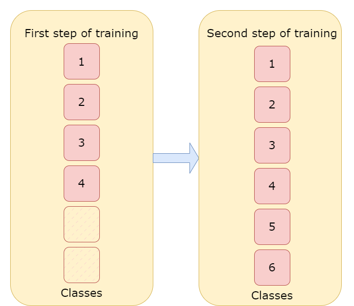
For the Curlicat data set, the training was made in two steps, firstly we trained our model on 4 classes with 100 samples per class and then made second training on 6 classes with 10 samples per class to check if the tested method can learn additional classes with few samples and avoid forgetting.

With the personal assistant data set, we made only one training on 16 classes with 10 samples per class, due to its simple structure.

The time we have to spend on training the model is difficult to estimate, due to the unstable nature of this method. However, the first stage is more predictable and repeatable and in our example, it took 2-3 hours to reduce the loss, but the second stage depends on the order of training samples can take from 1 hour up to 3-4 hours.

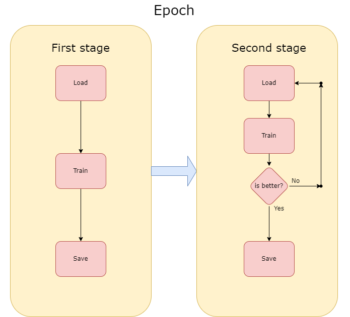
Additionally, each step had two stages. The method seems to be unstable in our case, despite low training loss, the validation prediction was very unstable, changing from 40% to 50% and then back to 40% or even 30%. To prevent this, we used stages. In the first stage, we are reducing training loss, saving the model for each epoch, but in the second stage, we are saving the model only if the F₁ metric from the current epoch is better than F₁ from the previous epoch. This solution let us train unstable methods to high prediction accuracy.

Results

To show our results we used accuracy and F₁ metrics. We tested the method on 100 samples per class in the first step and 300 samples per class in the second step. In the first step of training , we got 75% accuracy and 66.6% F₁, the method successfully recognized 3 out of 4 classes. In the second step, the few-shot learning step, we got 83,3% accuracy and 77,8% F₁ which is even better than the results from the first step and that leads us to a conclusion, we taught the model to learn. For the personal assistant data set with just one training on 16 classes with 10 samples per class, we got 70% F₁ while testing it using only the second step which is a similar result to the Curlicat

Potentially adjustments

One of the future adjustments can be changing the technique of adding new classes to the model. At this moment the place for new classes is reserved while creating the model which can lead to a situation when there won’t be a place for the new class. The solution is to make new places dynamically while adding new classes which can be done by modifying the classification layer, but while doing this we are losing our trained weights and that creates the need for second training with frozen weights which is very time-consuming.

Summary

This case gives us a clear view, that in some situations we don’t need thousands of records to successfully train models in machine learning and a few or a dozen samples can be enough. However, achieving high accuracy score can be challenging.

Resources

1. Chelsea Finn, Pieter Abbeel, Sergey Levine. ‘Model-Agnostic Meta-Learning for Fast Adaptation of Deep Networks’, 2017.
https://doi.org/10.48550/arXiv.1703.03400

2. Váradi, Tamás, Bence Nyéki, Svetla Koeva, Marko Tadić, Vanja Štefanec, Maciej Ogrodniczuk, Bartłomiej Nitoń, Piotr Pęzik et al. ‘Introducing the CURLICAT Corpora: Seven-Language Domain Specific Annotated Corpora from Curated Sources’. In Proceedings of the Language Resources and Evaluation Conference, 100–108. Marseille, France: European Language Resources Association, 2022.
http://www.lrec-conf.org/proceedings/lrec2022/pdf/2022.lrec-1.11.pdf.

3. Personal assistant

Author: Szymon Mielewczyk

Part 2: Abstractive text summarization – what’s it about?

Text summarization is the task of creating a new, shorter version of input text by reducing the number of words and sentences without changing their meaning and keeping their key parts.

There are many techniques for pulling out the most important data from input text but most of them fall into one of two approaches: Extractive or Abstractive. In this article, you will get the chance to get to know more about abstractive text summarization.

Models

Transfer learning, where a model is first pre-trained on a data-rich task before being finetuned on a downstream task, has emerged as a powerful technique in natural language processing (NLP). The effectiveness of transfer learning has given rise to a diversity of approaches, methodologies, and practices. If you are just starting with the task of text summarization you should know about BART and T5.

Before jumping into mentioned models let’s talk about BERT. This model was introduced in 2018 by Google. It is pre-trained to try to predict masked tokens and uses the whole sequence to get enough info to make a good guess. This works well for tasks where the prediction at position i is allowed to utilize information from positions after i, but less useful for tasks, like text generation, where the prediction for position i can only depend on previously generated words.

BART and T5 differ from Bert by:

Now let’s dig deeper into the big Seq2Seq pretraining idea!

BART

Documentation: https://huggingface.co/docs/transformers/model_doc/bart

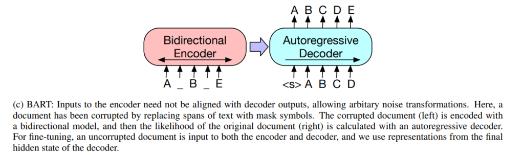
Figure from the BART paper

BART(facebook) is a well-known model used in many implementations of text summarization tasks. It is a denoising autoencoder using a standard seq2seq/machine translation architecture with a bidirectional encoder (like BERT) and a left-to-right decoder (like GPT).

Sequence-to-sequence format means that BART inputs and outputs data in sequences. In the task of creating summaries, the input consists of raw text data and pre-trained model outputs created summarization.

T5

Documentation: https://huggingface.co/docs/transformers/model_doc/t5

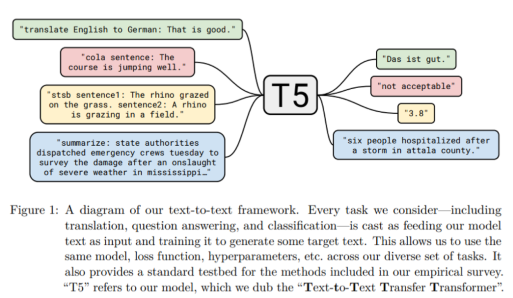
T5 Model Task Formulation.

T5 is a Text-to-Text transfer transformer model from Google. It is trained in an end-to-end manner with text as input and modified text as output. This format makes it suitable for many NLP tasks like Summarization, Question-Answering, Machine Translation, and Classification problems. Google made it very accessible to test pre-trained T5 models for summarization tasks, all you need to do is follow this tutorial to see how it works.

Let’s take a look at T5 models:

Google has released the pre-trained T5 text-to-text framework models which are trained on the unlabelled large text corpus called C4 (Colossal Clean Crawled Corpus) using deep learning. C4 is the web extract text of 800Gb cleaned data.

Google has released the pre-trained T5 text-to-text framework models which are trained on the unlabelled large text corpus called C4 (Colossal Clean Crawled Corpus) using deep learning. C4 is the web extract text of 800Gb cleaned data.

T5 expects a prefix before the input text to understand the task given by the user. For example, “summarize:” for the summarization. If you want to learn how to finetune a t5 transformer jump into this article.

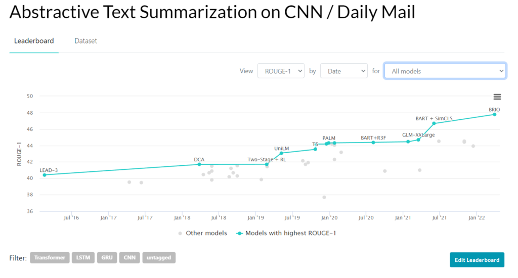
Besides learning about popular models like BART or T5 you will want to keep up with the newest models achieving SOTA. Papers with code has a whole page on abstractive text summarization. Leaderboards in the Benchmark section are used to track progress for this task.

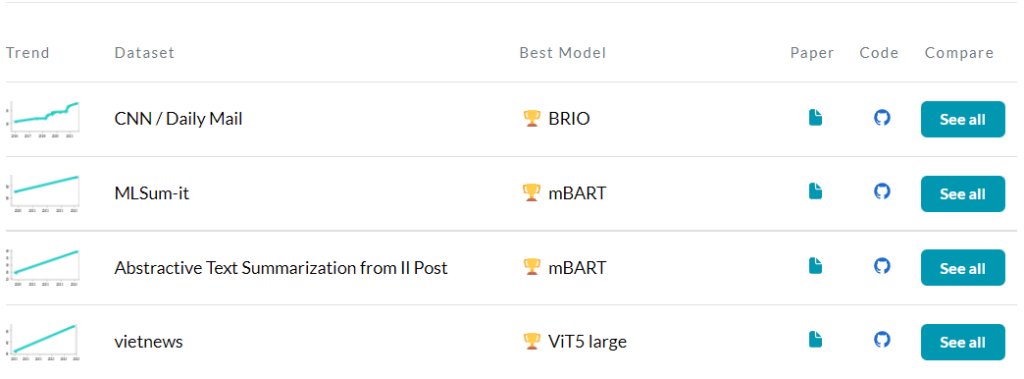
You can choose a Dataset and see results for some models and different metrics.

Pros and cons of abstractive text summarization

pros:

cons:

Datasets

You might have already heard some version of the quote “A machine learning model is only as good as the data it is fed”, Let’s explore this topic remembering how important it is for achieving a successful outcome.

At this point, we know a bit about existing models and where to find their documentation. You might have already tested some of them and now want to try finetuning one, but you don’t have your rich dataset? A good place to look for them is on papers with code. There are 41 datasets in total for this task.

If you want to take a look at some of the most popular ones jump into Part 1: Extractive summarization in a nutshell

Accuracy metrics and their challenges

As mentioned before measuring the quality of generated summaries can be complicated. The most common set of metrics used for measuring the performance of a summarization model is called the ROUGE score.

How does it work?

ROUGE score computes how much of the generated text overlaps with a human-annotated summary. The higher the score the higher overlap. It considers consecutive tokens called n-grams. In practice most commonly used versions are:

Sooo, what’s the problem?

This metric works well for getting a sense of the overlap but not for measuring factual accuracy. There are 2 unwanted scenarios:

Because metrics such as ROUGE have serious limitations many papers carry out additional manual comparisons of alternative summaries. Such experiments are difficult to compare across papers. Therefore, claiming SOTA based only on these metrics can be problematic.

In response to this issue there have been implemented new approaches:

Conclusion

This article covered all the main aspects of abstractive text summarization and a few popular challenges associated with it.

References

BART Docs:

https://huggingface.co/docs/transformers/model_doc/bart

BART: Denoising Sequence-to-Sequence Pre-training for Natural Language Generation, Translation, and Comprehension :

https://arxiv.org/pdf/1910.13461v1.pdf

Exploring the Limits of Transfer Learning with a Unified Text-to-Text Transformer:

https://arxiv.org/pdf/1910.10683.pdf

T5 Docs:

https://huggingface.co/docs/transformers/model_doc/t5

T5 models:

https://huggingface.co/models?search=T5

Tutorial for finetuning T5:

https://towardsdatascience.com/fine-tuning-a-t5-transformer-for-any-summarization-task-82334c64c81

Papers With Code | Abstractive text summarization:

https://paperswithcode.com/task/abstractive-text-summarization#datasets

To ROUGE or not to ROUGE?:

https://towardsdatascience.com/to-rouge-or-not-to-rouge-6a5f3552ea45

Entity-level Factual Consistency of Abstractive Text Summarization:

https://arxiv.org/pdf/2102.09130.pdf

Summarization of the above article:

https://towardsdatascience.com/entity-level-factual-consistency-in-abstractive-text-summarization-cb19e8a48397

InfoLM:

https://www.aaai.org/AAAI22Papers/AAAI-4389.ColomboP.pdf

Author: Alicja Golisowicz

Part 1: Extractive summarization in a nutshell

First of all: what is summarization?

According to Wikipedia text summarization “is the process of shortening a set of data computationally, to create a subset (a summary) that represents the most important or relevant information within the original content”. So, in short, it’s about extracting only essential information.

There are two main approaches: abstractive and extractive. Transfer learning with the use of transformers is a way to go in both.

In abstractive text summarization are used models such as T5 or BERT. After a proper training model is able to generate summaries based on given text.

On the other hand we have an extractive approach: localize the most important parts of the text and then combine them into a summary. In the end parts of the resulting summary come from the original text meanwhile in an abstractive solution model summarizes text with new phrases but keeping the point the same.

Advantages & disadvantages

To begin with, the main advantage is that sometimes (especially when we don’t have a good or big dataset) extractive summarization is a better option to choose because an abstractive approach can generate some fake information.

In terms of disadvantages: summaries can be stiff and repetitive, devoid of language grace. Also the overall quality highly depends on your data and model quality.

Datasets

First and the most difficult thing is to find the best suited to your needs dataset. Some sample datasets are available on Papers with code.

Let’s begin.

Which model?

Besides data we need a machine learning model to feed it. Training a transformer from zero is highly time & resource consuming. Fortunately, we have access to many models that require only fine-tuning to tailor your needs.

But what exactly is a transformer? If this question just popped out in your mind, please learn more in this post.

So, in terms of extractive text summarization the most popular one is a BERT: a transformer developed by Google, created and published in 2018. It’s a bidirectional transformer pretrained using a combination of masked language modeling objective & next sentence prediction on a large corpus comprising for example Wikipedia.

The original English-language BERT has two models:

Bert

Another powerful model is a T5 created in 2020 also by Google. It’s an encoder-decoder model pre-trained on a multi-task mixture of unsupervised and supervised tasks and for which each task is converted into a text-to-text format. Interestingly, T5 works by prepending a different prefix to the input corresponding to each task, e.g., for translation: translate English to German: …, for summarization: summarize: …..

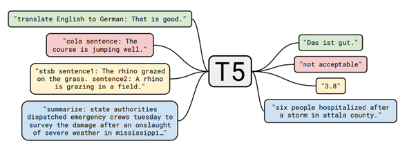
T5 tasks visualisation

If you wanna learn more check out papers with code.

Now when we have both the dataset and the model let’s begin training. But how do I know if my summaries are accurate or not?

Accuracy methods

The metrics compare our model-generated summary against reference (high-quality and human-produced) summaries. The most popular set of metrics to evaluate the quality of generated summary is the ROGUE.  Let’s take a closer look.

Reference: The kitten is tiny and cute.

Summary: Small kitten is cute.

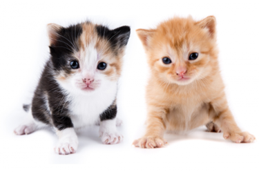
Kittens

ROUGE-N measures the number of matching n-grams between the generated text and a reference. For the ROUGE-1 precision will be computed as the ratio of the number of tokens in summary that are also in our reference: “kitten”, “is” and “cute”. Length of summary is 4, so the overall precision is 3/4.

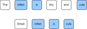
ROUGE-1 recall is inverted: it’s simply the ratio of the number of unigrams in reference that appear also in summary over the length of reference, so in our case: 3/6.

The ROUGE-2 can be calculated by analogy.

In fact the most used are:

Unfortunately ROUGE score does not manage different words that have the same meaning, as it measures syntactical matches rather than semantics.

How to do it?

In the approach presented in the paper  “Fine-tune BERT for Extractive Summarization”, when predicting summaries for a new document, we first use the models to obtain the score for each sentence. We then rank these sentences by the scores from higher to lower, and select the top-3 sentences as the summary.

For the example we’ll only select the top-1 sentence.

Sample text (from CNN/Daily Mail dataset):

[1] Never mind cats having nine lives. [2] A stray pooch in Washington State has used up at least three of her own after being hit by a car, apparently whacked on the head with a hammer in a misguided mercy killing and then buried in a field – only to survive.

[3] That’s according to Washington State University, where the dog – a friendly white-and-black bully breed mix now named Theia – has been receiving care at the Veterinary Teaching Hospital.

[4] Four days after her apparent death, the dog managed to stagger to a nearby farm, dirt-covered and emaciated, where she was found by a worker who took her to a vet for help.

So, the above data has 4 sentences. If we feed the model, the output can be:

[0.1; 0.5; 0.2; 0.2]

As we see, the second sentence scores the highest & it’ll be included in the summary.

This example has been simplified for ease of understanding by inexperienced persons. In the paper authors build several summarization-specific layers stacked on top of the BERT outputs, to capture document-level features for extracting summaries. These summarization layers are jointly fine-tuned with BERT. For the curious code is available here.

Summary

This article was an introduction to the task of extractive summarization. I hope it was a fun adventure 🙂 If you want to learn more, see Part 2: Abstractive text summarization.

Resources

https://en.wikipedia.org/wiki/Automatic_summarization

https://en.wikipedia.org/wiki/BERT_(language_model)

https://medium.com/nlplanet/two-minutes-nlp-learn-the-rouge-metric-by-examples-f179cc285499

Images

Bert: https://muppety.fandom.com/pl/wiki/Bert

Kittens: https://www.publicdomainpictures.net/en/view-image.php?image=167326&picture=cat-on-the-white

Author: Patrycja Biryło

An alternative lightweight fine-tuning strategy for Large Language Models using Adapter Fusion

Pfeiffer et al. (https://arxiv.org/pdf/2007.07779.pdf)

Motivation

The present language models like T5 or Bert are huge. The base version of T5 is reaching up to 220 million parameters and hundreds of megabytes of memory. Imagine how much time and resources-consuming is training a model like this. Fortunately, there is an idea of Transfer Learning, which means that authors – usually big tech companies and research centers – share their trained models. Everyone can easily download a pre-trained model and fine-tune on a specific task.

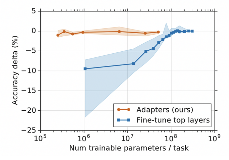
An alternative to fine-tuning is the idea of small task-specific layers called adapters. Adapter modules are characterized by compactness weighting from 0.2 to 4% of model size.

On the graph below we can clearly see that adapters perform as well as fine-tuning top layers despite having two orders of magnitude less parameters. Y axis at level 0 shows the performance of a fully fine-tuned model (all layers, not only the top layers).

Houlsby et al. (https://arxiv.org/pdf/1902.00751.pdf)

Some numbers, tests conducted by Houlsby et al. CoLA, SSt, etc are customary benchmark datasets in NLP area.

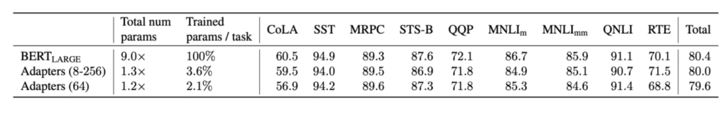
Houlsby et al. (https://arxiv.org/pdf/1902.00751.pdf)51.pdf)

Another important aspect where adapters and their fusion play an important role is the infamous phenomena of Catastrophic Forgetting, which will be explained in the third section.

What is adapter?

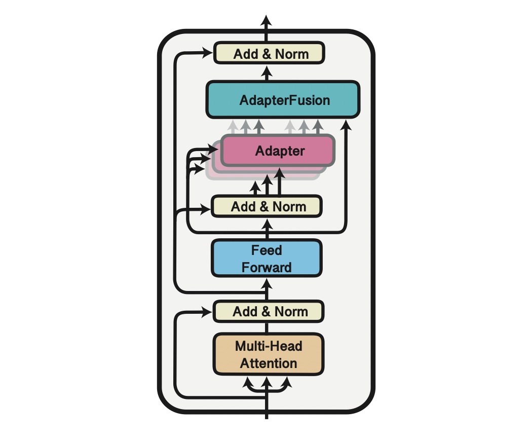
The idea of adapters in Transformers comes from Houlsby et al. (2019) in the paper „Parameter-Efficient Transfer Learning for NLP”. Originally, it consists of two small additional blocks inside the encoder layer in the Transformer architecture. During training we completely freeze the model’s parameters, leaving only adapters parameters to be trained.

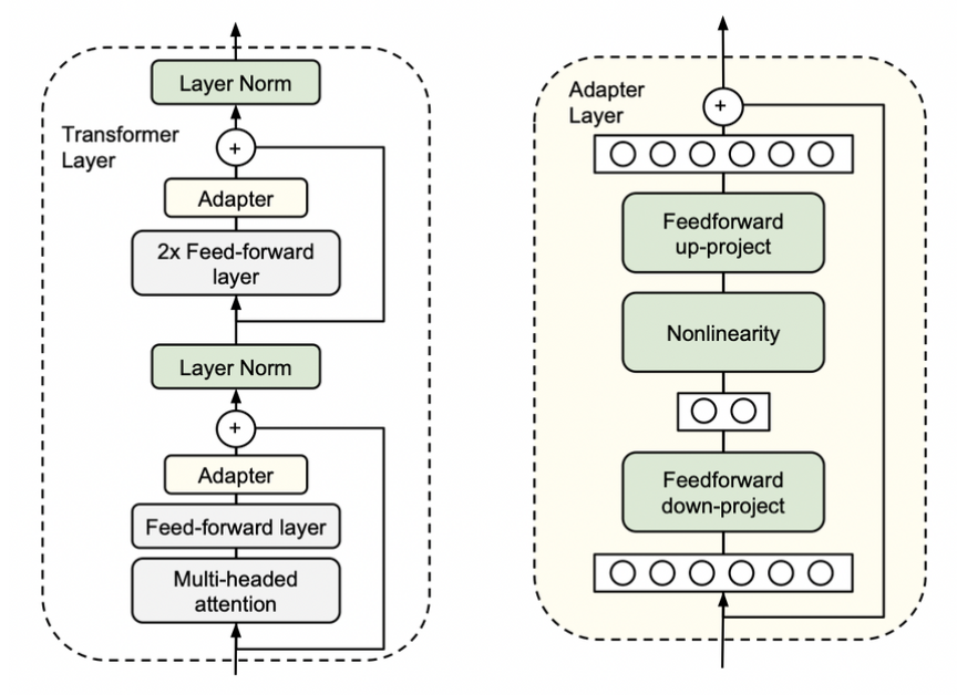
Houlsby et al. (https://arxiv.org/pdf/1902.00751.pdf)

The adapter is nothing more than another feature and information extractor with his „bottleneck” architecture. Processed data is projected to a lower dimension to filter only crucial information. After all, it is converted to the original size to match the model’s requirements. We call this configuration „Houlsby architecture” after the author. There are also different ideas with only one adapter layer, e.g., „Pfeiffer architecture,” which is lighter and the drop in performance is negligible.

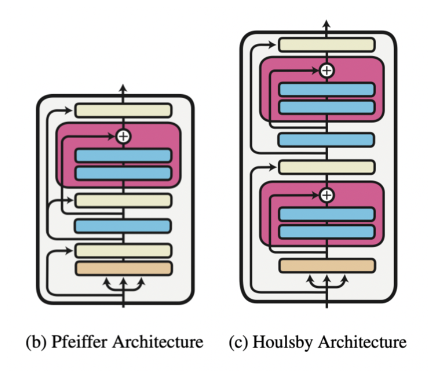
Pfeiffer et al. (https://arxiv.org/pdf/2005.00247.pdf)

Researchers and practitioners mostly use Houlsby architecture as it is based configuration and there is a hypothesis that lack of adapters in the last transformer layer is beneficial. Adapters in all encoder layers except the last one are encapsulated by frozen feed forward layers. It means they are separated from each other. Pfeiffer’s architecture in the last layers practically does not have an adapter as it is part of the prediction head. In contrast, Houlsby’s one has one adapter after a multi-head attention layer that is covered with a frozen feed forward layer above. Second is the extension of the prediction head.

The key idea is that an adapter works as an information extractor for a specific task, which will be crucial in the following section.

What is adapter fusion?

Once we know what adapters are, we can train a set of them each for individual tasks. The idea of fusion is to combine task-specific adapters with a single fusion layer that is similar to the attention layer. Both attention and fusion layers use the same equation and algorithm to calculate output.

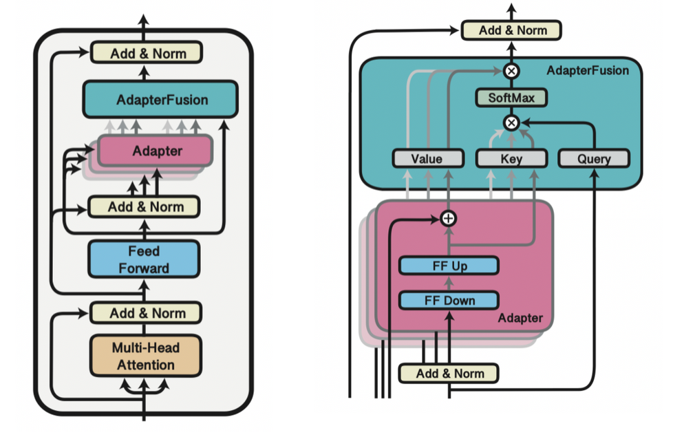
Pfeiffer et al. (https://arxiv.org/pdf/2005.00247.pdf)

This fusion layer learns to identify and activate the most useful adapter for a given input. The general rule is that adapters in lower layers are more generic, and thus are activated more often. In contrast, top-layer adapters are focused on details. Furthermore, Adapter Fusion extracts only information from adapters if they are beneficial for the specific task.

Adapter Fusion training can be divided into two stages.

Continual and Few-Shot Learning aspects

Continual aspect of learning focuses on situations where we have trained a model and, after some time, the new data with different distribution. In a fine-tuning regime, we would have to re-train our model with all the data gathered. It would not only be very time-consuming but also, as the model learns new patterns, the weights are overwritten. It leads to forgetting the previous knowledge. This phenomenon is called Catastrophic Forgetting.

Adapters help avoid this common pitfall of multi-task learning. New adapters learn knowledge for new tasks, and old ones do not have to be overwritten. Fusion combines adapters, learning which and when each adapter should be activated.

Sometimes we are forced to work in a regime of a small amount of data – a Few-Shot scenario. This is another aspect where adapters fits well thanks to its relatively small architecture. In the next section, we will see how they perform on a small dataset.

Adapter Fusion in action!

We are going to implement adapter fusion with the Bert model using Pytorch and the transformers library. [1]

We will download and load the CommitmentBank (De Marneffe et al., 2019) dataset.

from datasets import load_dataset
dataset = load_dataset("super_glue", "cb")
print(dataset.num_rows)
-> {'test': 250, 'train': 250, 'validation': 56}

This dataset has 556 examples, each of which contains a premise and a hypothesis. The objective is to classify the relationships between them. Whether it is 'entailment’, 'contradiction’, or 'neutral’.

The first step is to encode data for the selected Bert model (bert-base-uncased from hugging face).

from transformers import BertTokenizer 
tokenizer = BertTokenizer.from_pretrained("bert-base-uncased") 
def encode_batch(batch):
    """Encodes a batch of input data using the model tokenizer.""" 
    return tokenizer( 
         batch["premise"], 
         batch["hypothesis"], 
         max_length=180,
         truncation=True,
          padding="max_length") 
# Encode the input data
dataset = dataset.map(encode_batch, batched=True) 
# The transformers model expects the target class column to be named "labels" 
dataset = dataset.rename_column("label", "labels") 
# Transform to pytorch tensors and only output the required columns
dataset.set_format(type="torch", columns=["input_ids", "attention_mask", "labels"])

After that, we can create an instance of Bert with the proper configuration and labels.

from transformers import BertConfig, BertModelWithHeads 
# Preparing labels equivalent 
id2label = {id: label for (id, label) in enumerate(dataset["train"].features["labels"].names)} 
config = BertConfig.from_pretrained( 
                 "bert-base-uncased",
                 id2label=id2label, 
)
 model = BertModelWithHeads.from_pretrained( 
                    "bert-base-uncased", 
                    config=config, 
)

Later, we can add adapters (we use pre-trained from adapterhub) without classification heads and activate them. All of them are in Houlsby configuration and were trained on different task-specific datasets:

On top of that, we add an adapter fusion layer and cover it with a randomly initialized classification head which we call „cb”.

from transformers.adapters.composition import Fuse
 
# Load the pre-trained adapters we want to fuse 
model.load_adapter("nli/multinli@ukp", load_as="multinli", with_head=False)
model.load_adapter("sts/qqp@ukp", load_as="sts", with_head=False) 
model.load_adapter("nli/qnli@ukp", load_as="nli", with_head=False) 
# Add a fusion layer for all loaded adapters 
model.add_adapter_fusion(Fuse("multinli", "qqp", "qnli")) 
model.set_active_adapters(Fuse("multinli", "qqp", "qnli")) 
# Add a classification head for our target task 
model.add_classification_head("cb", num_labels=len(id2label))

It is time to freeze the model and adapters parameters. Only fusion layers need to be trained.

# Unfreeze and activate fusion setup
adapter_setup = Fuse("multinli", "qqp", "qnli") 
model.train_adapter_fusion(adapter_setup)

The last step is to prepare the evaluation metric and the training part.

import numpy as np from transformers
import TrainingArguments, AdapterTrainer, EvalPrediction
training_args = TrainingArguments( 
                      learning_rate=5e-5, 
                      num_train_epochs=5, 
                      per_device_train_batch_size=32, 
                      per_device_eval_batch_size=32, 
                      logging_steps=200,
                      output_dir="./training_output", 
                      overwrite_output_dir=True,
                      # The next line is important to ensure the dataset labels are properly passed to the model 
                      remove_unused_columns=False, 
)
def compute_accuracy(p: EvalPrediction): 
   preds = np.argmax(p.predictions, axis=1)
   return {"acc": (preds == p.label_ids).mean()}
trainer = AdapterTrainer(
                model=model, 
                args=training_args, 
                train_dataset=dataset["train"],
                eval_dataset=dataset["validation"],
                compute_metrics=compute_accuracy, 
)
# Train model
trainer.train()

Then we can evaluate our model after fusion, reaching up to a 71% accuracy score!

print(trainer.evaluate())
 -> {'eval_loss': 0.7297406792640686, 
     'eval_acc': 0.7142857142857143, 
     'eval_runtime': 1.1516,
     'eval_samples_per_second': 48.628, 
     'eval_steps_per_second': 1.737,
     'epoch': 5.0}

Summary time

As we have seen, Adapter Fusion is an interesting compact method of Transfer Learning. Reaching nearly SoTA results but with much less effort and time. In addition to this, they perform well in the Few-Shot and Continual Learning regimes and are able to face Catastrophic Forgetting problem.

Resources

[1] – https://colab.research.google.com/github/Adapter-Hub/adapter-transformers/blob/master/notebooks/03_Adapter_Fusion.ipynb

Author: Beniamin Sereda

Classification of customer complaints based on data from the Consumer Financial Protection Bureau.

Business overview

Knowing the customer is the success key of marketing. Enterprises collect more and more customer data. They do it openly or covertly. Sometimes, when asked about the quality of service, the company wants to discover what its client needs and adjust the offer accordingly.
It is related to high competition and the desire to match the offer in the best possible way.

The matter of customer data analysis is a very complex issue that concerns many industries. One of the types of data with high added value is complaints submitted for services or products.
The purpose of this task is to categorize company complaints using machine learning. Thanks to this, it will go to the appropriate department and be resolved faster.

Data overview

Since the topic is very extensive we decided to analyze the complaints data from Consumer Financial Protection Bureau, a federal agency from the USA. They were downloaded from the official website, written in English, and include complaints about consumer financial products and services that the CFPB has sent to companies for response. The dataset contains more than 4 years of customer behavior in this area (the first data points are from 2017). In total, 28,864 anonymized complaints with their metadata were collected.

Data preprocessing

During the data analysis, only the isolated columns that were most important to the process were worked on: product, issue, subissue, narrative.
The complaints concerned the following products:

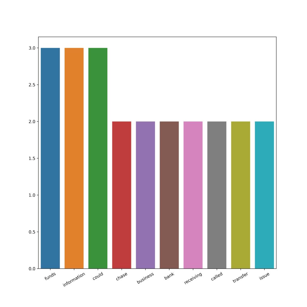
As part of data processing, the NLTK library was used. Dataset was tokenized and stopwords, numbers, and missing data were removed. Most of the top 20 tokens are what can be considered a stop word.
Also, the frequency analysis was performed. The most common words are ex.: account, report, credit, verified.

The main categories of the product were also renamed to make the names easy to type.
Mortgage and loans were combined because of the small frequency. Also, a set of information considering the complaint was joined together to have full information about a complaint. An example one is as follows:

Hello This complaint is against the three credit reporting companies. XXXX, XXXX XXXX and equifax. I noticed some discrepencies on my credit report so I put a credit freeze with XXXX.on XX/XX/2019. I then notified the three credit agencies previously stated with a writtent letter dated XX/XX/2019 requesting them to verifiy certain accounts showing on my report They were a Bankruptcy and a bank account from XXXX XXXX XXXX.

Modelling Pipeline

As the very first step to modeling vectorizing with TF-IDF (with max_features= 5000000) matrix was introduced. Also, the data was transformed by CountVectorizer as the second experiment. Lemmatization using WordNetLemmatizer was performed.
Before actual modeling, the matrix was divided into a training set (80%) and a testing set (20%). The product remained the target variable.

product	narrative
0	retail_banking	wife wired money personal account joint chase …
1	debt_collection	today individual sheriff department delivered …
2	credit_reporting	hello complaint three credit reporting company…

The following types of models were tested:

At first with default parameters, then with a few parameter selections.
The best result was achieved using Decision Tree with Count Vectorizer:
Accuracy: 94.5%
Precision: 95.4%
Recall: 75.9%
F1: 79.8%

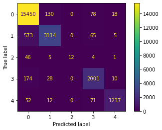
Also, due to imbalanced classes SMOTE was introduced. All models gave similar results between training and testing sets, which would mean that they didn’t overfit the data.
The second closest from the best was KNN:

Accuracy: 87.7%
Precision: 67.7%
Recall: 60.9%
F1: 63.8%

Comments

It is worth noting that one of the greater limitations of this task is the amount of data, or rather the number of variables, that is created for the text. In the case of models whose quality can be improved by searching for hyperparameters, these are already one-hour processes. Another point is that this is typical of a text analysis case.
The above task proves that free text machine learning can be very beneficial for the enterprise. The ability to automatically classify incoming documents saves a lot of money on the human factor. The models that were developed as first attempts are decent.

Author: Karolina Wadowska