

Natural Language Processing
Generating paraphrases
Generating paraphrases

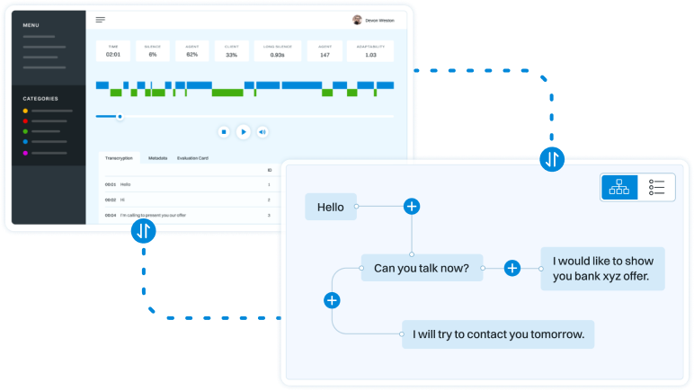
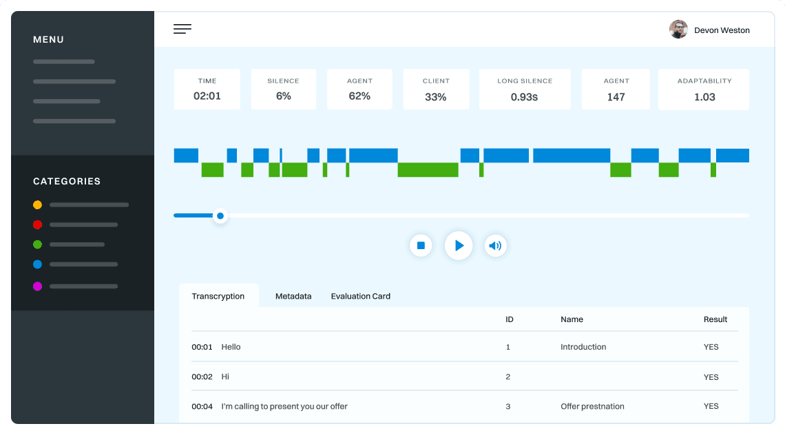
TRURL brings additional support for specialized analytical tasks:
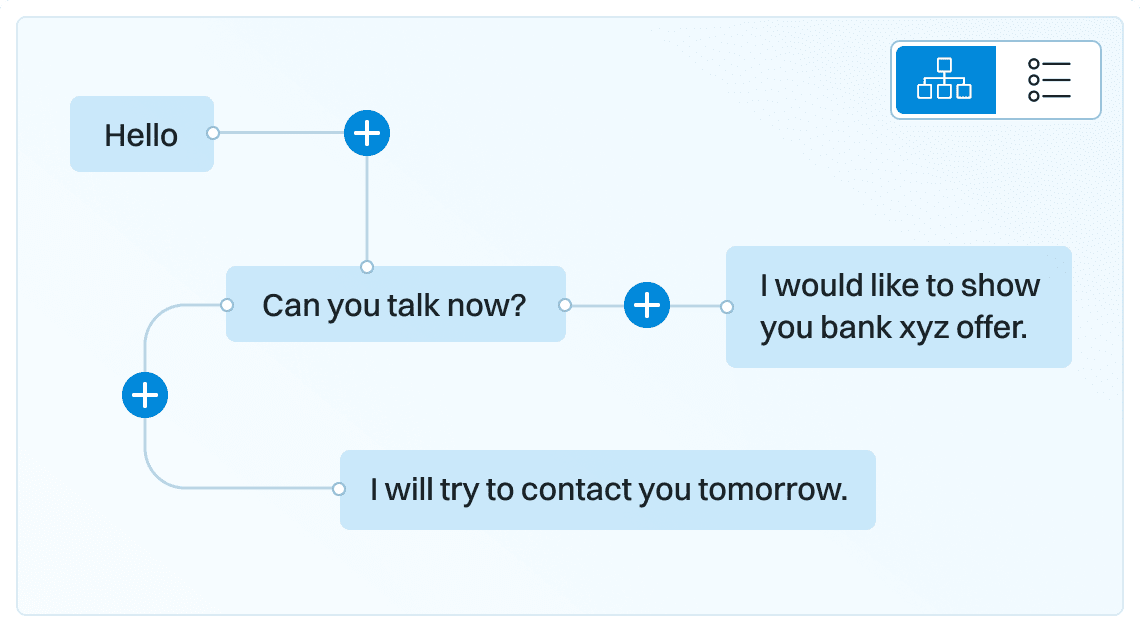
Dialog structure aggregation
Customer support quality control
Sales intelligence and assistance
TRURL can also be implemented effectively on-premise:
We will build a GPT model for you
Trained securely on your infrastructure
Trained on your dataset

Share
Data is the key ingredient in Machine Learning, which is based on learning from it. The Deep Learning field is even more data hungry, due to large models, that need to generalize well and avoid overfitting to the training data. In most Machine Learning problems like Speech Recognition getting large amounts of labelled data is very expensive and time-consuming. This was discussed in a previous blog post on self-supervised trend in Speech Recognition (link). The self-supervised paradigm is pretty recent, but very promising method used in Speech Recognition (link). Another method, that was used even before the Deep Learning era is Pseudo Labelling (link, link, link, link). This is a Semi-Supervised learning paradigm, which uses model’s own output labels to train itself.
The standard procedure is to predict the labels for the unlabelled data and filter those, which prediction probability is pretty low. This should leave only examples, which in most cases are correctly labelled. How well this technique works is highly dependent on the models quality and how trustworthy are the probabilities. For tasks, where the output is not a single label, but a sequence such as Speech Recognition there is another problem, which is how to handle examples, when part of it is pretty confidently recognized and part has much worse probability. An example could be a single-channel agent-client phone conversation, where client’s speech is often of much worse quality. It is important to notice, that the agent’s voice has much better quality, but the client’s is adding much more to the speaker and domain variability. To improve the filtering quality the pseudo labels could be checked for some model specific errors (link). During the process the hard examples are being filtered-out. Similiar to supervised training to make the data more useful the model need to be disrupted with some regularizations, like dropout, or data need to be augmented with noise or SpecAugment (link, link) to get more out of it.
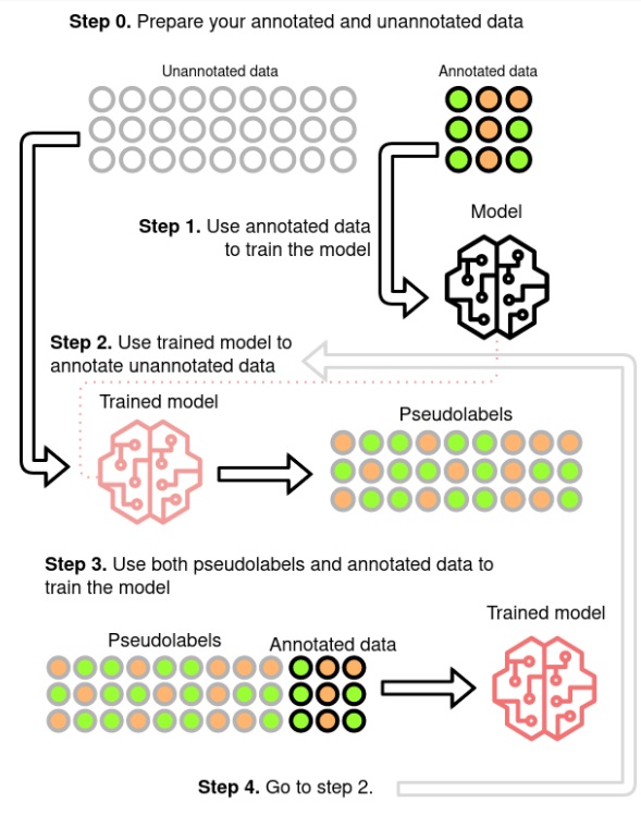
Pseudo-labeling method (source)
Having improved the model in a Pseudo Labelled setup the question that arises is if the model, being learned on the unlabelled data, could create a better pseudo labels for it, than the fully supervised one. This was explored in (link) as Iterative Pseudo Labelling and in (link) as Noisy Student Training. Both state that data augmentation, beam-search decoding with an external Language Model (LM) and balance between the labelled and unlabelled sets are the keys for good performance. (link) uses also filtering mechanism, which probably leads to the better results. In both approaches the beam-search decoding and the external LM are the most problematic components. Beam search, because it is computationally expensive, limiting the number of iterations. External LM, because it is biasing the Acoustic Model (AM) (link). (link) proposes Language-Model-Free IPL (slimIPL) rejecting the beam-search and LM, by using the most probable AM outputs combined with a dynamic cache. Using the dynamic cache enables part of the unlabelled examples to be processed again in a short period with the same pseudo labels and it was shown that this greatly increases the stability of the training, especially for experiments with small labelled sets. The instability is most often caused by model pushing itself into outputting ever less labels. Having generated labels only for a part of the true labels, it is encouraged through learning on them to omit even more. Dynamic cache probably by showing the same example again with more labels than the current model would generate is stopping the model from taking that path. There were proposed alternative approaches to stabilize the training using exponential moving average (EMA) (link, link). One of them was even shown to effectively combine with the dynamic caching.
Most of the articles’ experiments are performed on the Librispeech dataset (link), sometimes adding LibriLight (link) for large scale experiments. The dataset consists of audiobook recordings read by voluntary speakers. This gives often not very high quality audio and lot of accents, but they are single speaker recordings of rather static intonation and speed, containing little emotions and background noises. With current SOTA Speech Recognition models (link) it is possible to achieve 1.9% WER for clean and 3.9% for other test sets without any unsupervised or semi-supervised approaches. This brings doubt if the semi-supervised methods could perform well on real-life data. (link) tests the slimIPL on Conversational Telephone data, but those popular sets (Switchboard (link), Fisher (link, link)) can be classified as single source (single domain). Combining multiple models it is possible to achieve even 5% WER on the corresponding test set, which is not achievable on real-world telephone data (link) (the authors stated on Interspeech 2017 presentation that real-world data had ~20% WER on this model). (link) uses public videos as training data for English and Italian. It is hard to judge the quality of the data, but the semi-supervised approach gives almost same results using only 10h of labelled data and 75kh of unlabelled compared to 650h labelled data in supervised training, which makes the acoustic models creation much faster and cheaper. So it is not exactly clear how the Pseudo Labelling would perform if the labelled data would be of much different acoustic domain than the unlabelled or if the unlabelled would come from lots of acoustic domains.
In our Pseudo Labeling experiments we used modified version of Performance Monitoring (link) to filter out the audio files that are predicted to have worse WER than a threshold. It is working well for high quality audio like data from media. The correlation between predicted WER and real WER is pretty good, but when used for lower quality 8kHz telephone data the WER correlation is not good enough. Experiments with such data show, that the resulting model is performing worse than a model on labeled data only.
Inferring from our experiments and from articles one can state, that the Pseudo Labeling approach is working well if the data is of high quality and the model can predict labels with pretty high accuracy. If the quality of the audio is lower and even the human error is pretty high, the recognitions will give lots of errors, so for some corpora the pseudo-labelled data can bring more harm than good. The second argument against using it for telephone data is the data augmentation. As for SpecAugment it can be accepted that it does not shift the domain of the data, but adding noise could be seen as such shift. So the best way to improve for such data would be augmenting a better quality to an approximation of the telephone quality, but such a domain shift is a separate research area by itself.
In comparison to Self-Supervised learning Pseudo Labelling seems to be less computationally expensive (slimIPL’s 83.2 vs Wav2Vec2.0’s (link) 294.4 GPU-days)(link), but if working on multiple languages probably this would shift on the other side, because of easier reusability of the pre-trained Self-Supervised model. A great news is that the slimIPL can be combined with models like Wav2Vec2.0 and adds additional value on top of them (link, link). As for the multilingual usage a procedure was proposed (link), but compared to Self-Supervised training it is a pretty complex one.
So the Pseudo Labelling approach is best suited if one stays in a relatively closed domain and has lots of real-life data of decent quality. The good thing is that it could be setup in a self-learning mlops manner, that is continuously improving by combining the available labelled data with new incomming production data. This should improve the model both generally, but especially for the new domains that will appear. To enhance the process part of the most difficult filtered-out examples could be sent to the human-in-the-loop and come back as labelled data improving also for the worst quality data.
Share
Author: Jakub Kaliski
Share
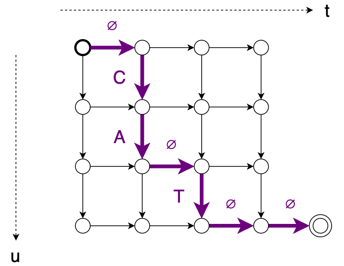
Connectionist Temporal Classification(CTC)(link) is one of the most popular criterion in Speech Recognition. It brings both good performance and training simplicity, but one of main disadvantages is conditional independence of labels. Another one is requirement for input to be longer than output. RNN Transducer (RNNT)(link) was proposed to overcame those issues. New loss function expands CTC mechanisms – blank label and time-restricted alignment, presents some new improvements, and removes inconveniences.
To address first problem, RNNT introduces new model architecture consisting of Predictor Network combined with Encoder Network in Joiner Network.

Encoder behaves as acoustic model – produces latent representation of acoustic features. Predictor consumes sequence of text tokens, thus can be seen as inner Language Model. Joiner sums both modules outputs and proceeds with simple feedforwad layer transforming latent representation to output labels probability distribution. The main idea is to support acoustic part of speech recognition with lexical dependencies built on recognition history. Both Encoder and Predictor network can be transferred from pretrained models – CTC, CE or other tasks, like wav2vec, can be utilized as Encoder while Predictor can be initialized with Neural language Model. RNNT operates in time and labels space, thus allows multiple outputs for single input, which solves second problem.
Incorporating Predictor Network can be beneficial not only in terms of modeling capability. Since Predictor operates purely on text input, it can be easily pretrained on large amount of data. Predictor can also be adapted to new domain using this mechanism (link, link). In contrast to audio, large amount of text data suitable for training are easily available. It also allows to make use of user data, ie on contact list on mobile device. Such single module adaptation can be performed directly on device, assuring privacy.
Unlike standard Attentions models, RNNT can run in streaming fashion, even on mobile devices (link). Seq-2-Seq models tend to relay on full input sequence. It is possible to restrict their inference to current(or contexted) input, but it has impact on performance. In contrary, RNNT itself does not model time dependencies, thus can run in streaming fashion out of the box. Forcing Seq-2-Seq models may also bring noticeable delay into system. RNNT model latency can be controlled in multiple ways – with loss function restrictions utilizing alignments (link) or forcing monotonic outputs, decoding strategies (link) or auxiliary losses (link). RNNT seems to work well with wordpieces outputs (link, link), which helps to keep good realtime and computational complexity by reducing output steps number.
With all this features come some drawbacks. The most severe one is training memory consumption. Since acoustic and text representation can vastly differ in length, they cannot be simply added. We can combine two 3D matrices using broadcasting, but it forces huge memory overhead due to spare paddings (link). Keep in mind it’s only forward pass, we need to keep parameters for backpropagation as well. Alongside common ways of reducing memory footprint, like using half precision or training using examples sorted by length, some new techniques were proposed. Broadcasting was replaced with per utterance combination (link) followed by concatenation, so there is no extra padding added to shorter examples. The same article utilizes merging softmax function into loss computation, which can save extra memory when using large amount of wordpieces. Recently k2 project team put their effort to optimize RNNT memory footprint. They implement some of already proposed solutions (Recurrent Neural Aligner – restricted varaint of RNNT so it can emit only one symbol per frame), as well as some new ideas, like pruned RNNT. This approach minimizes memory usage by pruning zero gradients from backproagation.
Also predictor can introduce some exposure bias to model – training on small amount of data may lead to overfitting and generalization issues. Some methods to prevent this aim directly at training procedure (link), while other propose architecture changes (link) or training pipeline tricks (link). With all mentioned above, RNNT models can be challenging to train and diagnose.
Despite problems, RNNT seems to gain more and more attention, and list of frameworks offering RNNT keeps growing. Here are some of them:

NeMo (link)
SpeechBrain (link)
PyTorch (link)
k2 (link)
ESPnet (link)
There are some standalone implementations offering bindings to popular libraries like PyTorch or Tensorflow (link). Surprisingly, there is no official implementation in Tensorflow, despite Google seems to put some effort in RNNT development (link). Efficient RNNT implementations from k2 are available as separate modules (link).
Combining all together, we think RNNT can lead to further speech recognition improvements. Incorporating lingual aspect directly into acoustic model may boost generalizing abilities, especially in challenging acoustic conditions. Predictor adaptation using only text data may be easy way dealing with new/out of domain data. Keep in mind, that so far we only considered ASR systems without external Language Model. While in conventional systems, Language Model integration is quite straightforward, RNNT offers few strategies of fusion, like deep, shallow or cold. (link)
It seems that RNNT can lead to SOTA results in some products, like mobile devices systems or streaming applications. Modular design allows to use pretrained Encoder and Predictor networks as single pipeline in end-to-end manner and greatly simplify speech recognition system. With more attention from research teams, RNNT will improve in field of memory footprint, training stability and overall performance.
Share
Author: Jakub Filipiuk
Share
Self-supervised pre-training is one of the most promising methods in the deep learning field. Following Computer Vision and Natural Language Processing, it recently became one of the most popular topics in Automatic Speech Recognition (ASR) research. The proposed Contrastive Predictive Coding (CPC) (link) has shown great potential in using unlabeled data for Phone and Speaker Classification. This has now marked the start of a huge effort led by the big tech companies to utilize the most out of the ocean of unlabeled speech data that is currently available on the Internet.
The reason why this is such an appealing topic is due to the large financial cost of labeling large amounts of speech recognition data for use in the training of Speech Recognition Systems. Current commercial ASR corpora can cost up to a few hundred dollars per hour of data. Examples include the American English Speech Recognition Corpus (Mobile) from ELRA (link), which costs 6000€ for 14.67 hours of speech. Combined with the observation that in order to reduce the Word Error Rate (WER) by 50% for a neural network model (link) the dataset must increase by a factor of 10, we come to the conclusion that it is only feasible to do achieve a certain WER, after which the returns are diminished by the financial cost of buying or labeling new data. Furthermore, achieving a satisfactory WER via datasets of transcribed audio is only practical for the most commonly spoken languages, where the client base is much greater. For this reason, big tech companies and the rest of the industry have been focused on finding different, more scalable solutions.
Since the original CPC article and its extension wav2vec (link), which was the first to show its ability to achieve comparable state-of-the-art (SOTA) results on a commonly used dataset, there has been a wave of articles and research further adding and expanding upon the original work, combining it with some existing research or simply using it for other tasks or domains. The most important work uses wav2vec2.0 (link), which beat the SOTA results on the LibriSpeech (labelled) + LibriLight (unlabeled) datasets. This was achieved by using another promising method: Noisy Student Training (link), also known as Pseudo Labelling (link), which we will cover in a separate post soon. The best feature of the two methods is the fact that they can be successfully combined (link, link), with the main drawback of the wav2vec2.0 versus CPC or wav2vec being that it uses a large full context Transformer model and a masked based training procedure, so it cannot be used in a low-latency ASR system.
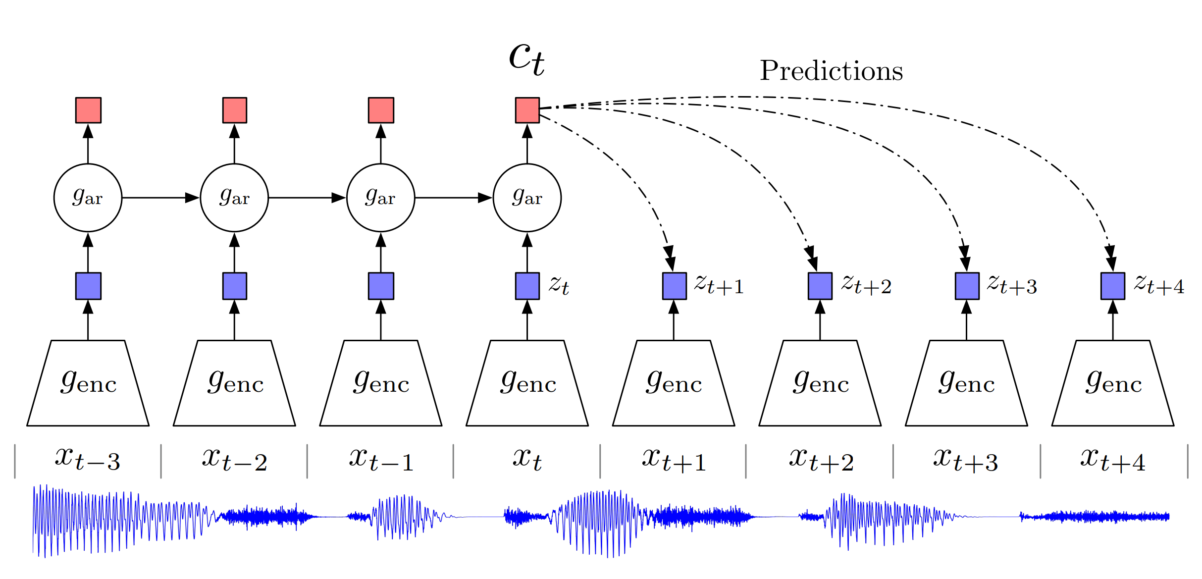
Overview of Contrastive Predictive Coding, the proposed representation learning approach.
Although this figure shows audio as input, we use the same setup for images, text and reinforcement learning. (source)
The main idea in self-supervised learning is to learn some kind of representation of the input signal that can be useful for the downstream task. To do so, we need to define a loss function that can learn something meaningful. Both the original CPC and wav2vec2.0 losses are inspired by the losses used in language modelling. The Recurrent Neural Network Language Models (link) were trained to predict the next word having the current word as input and all previous words as context. This paradigm forces the neural network to learn a representation of each word and their combination to be able to predict which next words are making sense in this context, thus learning the structure of a language purely by receiving lots of text data, which is very easy to attain in large quantities. Having such a pre-trained model, one can fine-tune it to a more precise task where the data is much sparser, such as Text Classification (link). The same goes for CPC, but due to the unclear boundaries of a speech signal, its variability and sample density (usually 8k or 16k per second), a latent signal representation is needed to make the prediction task a reasonable one. This introduces the problem a new problem to the model, wherein it may simply “collapse” by zeroing out the latent representation and achieving a 100% accuracy rate. To prevent this, the contrastive task was proposed: to distinguish following frames from N randomly sampled ones, which forces the representations to differ. As the speech signal can stay longer in some phonemes than in others, in order to give more incentive to learn, the model is set to predict more than one succeeding latent representations, preventing it from making a simple prediction that the latent vector will always stay the same because it should be true for a significant portion of the time. Combining this has given the authors a method to successfully train a model which achieved promising results on both Phone and Speaker Classification tasks. The following wav2vec proved that it is useful as pre-training of Acoustic Models (AM) for ASR.
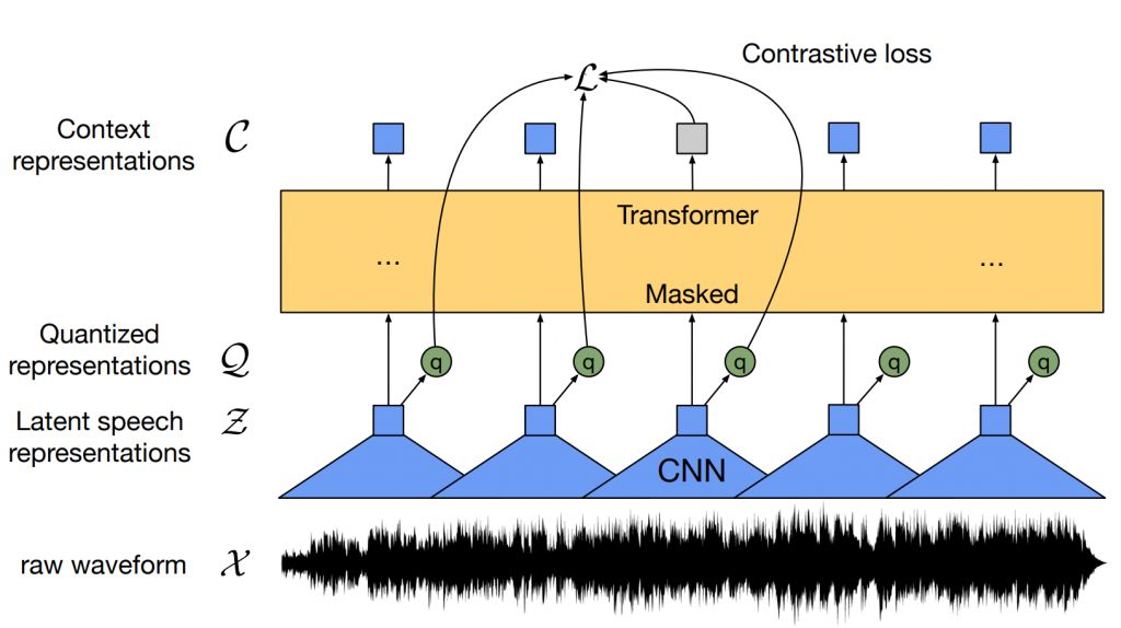
Illustration of framework which jointly learns contextualized speech representations
and an inventory of discretized speech units. (source)
The wav2vec2.0 was inspired by the BERT model (link), where having a model that needs a full future context the prediction of the next token was infeasible. To mitigate this, Masked Language Modeling (MLM) was proposed where some input tokens are masked and the model has to predict them. In wav2vec2.0 the model is trained in the MLM fashion, but on the quantized latent representations. This forces the use of contrastive loss, Gumbel SoftMax (link), and a diversity loss (link) to encourage the usage of all classes. The use of powerful Transformers and MLM-like procedures has enabled valuable pre-training and reduced the need for labelled data, giving great results also for other languages that were not included in the pre-training (link). Further research tries to add something on top of this, such as offline clustering of similar frames to discover hidden units in HUBERT (link), additional loss functions (link, link), which brings some small gains or more robustness in some domains or simply scaling (link). The big problem in these models is the cost of the pre-training, which for the original wav2vec2.0 was around 16000 GPU-hours [5], as well as its instability (link, link). So taking all data you can get and throwing it into the model is not the best idea. Besides, although the models are great for in-domain data, when faced with some domains that are further apart from the data used in pre-training it does not so well (link). The proposed remedy is to do a pre-training continuation on the target domain data, which gives large WER reduction even if the fine-tuning data is not in the target domain, but still requires a lot of the unlabeled target data to really make a difference. So, in terms of generalization, the speech community still has much to discover, even outside the pure self-supervised training domain (link).
Self-supervised pre-training is a great effort to make speech recognition more available for the less spoken languages, especially due to the openness of the big companies and the machine learning community, which provide models with their research. If this were not the case, pre-training such models would be unachievable for most researchers and small companies due to the enormous GPU computational cost. Still, moving outside of the target domains brings lots of challenges in and of itself. Furthermore, as the research progresses into ever larger models (link) we will soon face Megatron-Turing NLG-like (link, link) sizes, which will only be attainable for companies with large financial means. In summary, despite the fact that hardware is improving by great leaps and bounds, what most needs improvement are the methods used to train such enormous models, preferably to reduce them to only a fraction of the computational cost that they have today. Hopefully, some breakthroughs in this matter will be coming soon.
Share
Author: Jakub Kaliski