

Natural Language Processing
Generating paraphrases
Generating paraphrases

TRURL brings additional support for specialized analytical tasks:
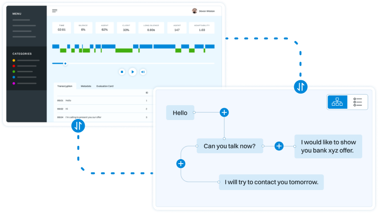
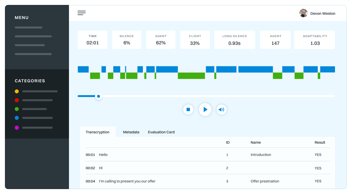
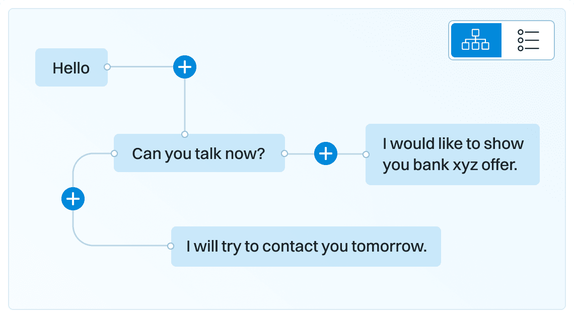
Dialog structure aggregation
Customer support quality control
Sales intelligence and assistance
TRURL can also be implemented effectively on-premise:
We will build a GPT model for you
Trained securely on your infrastructure
Trained on your dataset

Share
One of the crucial tasks in language understanding is topic modeling. Our highly abstract minds grasp topics quite easily. We naturally understand a conversation or written text context. But what exactly is a topic?
According to Cambridge Dictionary a topic is:
a subject that is discussed, written about, or studied.
Topic modeling focuses on preparing tools, models, or algorithms that might help discover what subject is discussed by analyzing hidden patterns. Those topics models are frequently used to find topics changes in the text, web-mining, or cluster the conversations. It is an excellent tool for information retrieval, quick large corpora summarization, or a method of feature selection. For instance, in Voicelab, we use topic modeling to categorize texts and transcripts quickly and discover inner patterns in conversations.
Below, there is an example of analysis of hundreds on conversations
with our topic sensitive kwT5 model.

However, to train such models, we need data. Lots of data. There are a few ways to approach this. Some experiment with supervised learning — but old-school supervised training requires manually labeled data. But some approaches don’t require annotated data (unsupervised learning). For instance, researchers tried to generate word or sentence embeddings using pretrained language models like BERTs or Word2Vecs and then to cluster them. Some used statistical methods like Latent Dirichlet Allocation (LDA) that represents documents as mixtures of topics that spit out words with certain probabilities. Others use approaches like KeyBert. KeyBert extracts document-level (or conversation-level) representations and uses cosine-similarity to compare them with the most similar words in the document. This allows for extracting key-phrases that are often closely related to the subject of discussion.
Those are nice but still not perfect. BERTs work great, but their pretraining process is not designed for topic modeling. And LDA is not that good with catching more difficult abstract concepts. Here is when the self-supervised approach comes to the rescue.
This type of learning uses unlabeled data and creates a pretext task to do. For instance, we can take a large corpus and try to predict the next word for a given sentence. Or we try to remove a single word and try to predict it. Usually, in each pretext task, there is part of visible and part of hidden data. The task is either to predict the hidden data or predict some property of the hidden data. So why not try to specify a pretext task closely related to the topic modeling?
The pretext task is the self-supervised learning task solved to learn meaningful representations, to use the learned representations or model weights obtained in the process, for the downstream task.
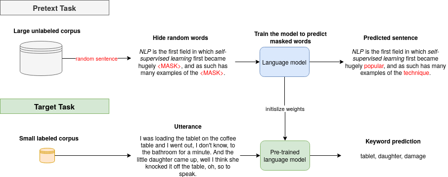
Learn more about pretext tasks here.
As we already know what a pretext task is, let’s focus on the topic-specific task for pretraining our NLP models. In 2019, an exciting model was proposed using Siamese BERT models for the task of semantic textual similarity (STS).
Semantic textual similarity analyzes how similar two pieces of texts are.
The paper uses a vast, open, and well-known text corpus available in multiple languages: Wikipedia. Wikipedia articles are separated into sections that focus on specific aspects. Hence, sentences in the same section are thematically closer than sentences in different sections. This means that we can easily create a large dataset of weakly labeled sentence triplets:

The anchor (base sentence)
The positive example coming from the same section
The negative example from a different section
All examples in a single sample should come from the same article.
For instance, let’s look at a NLP article in Wikipedia.
Let’s take an anchor from the History section:
Up to the 1980s, most natural language processing systems were based on complex sets of hand-written rules.
And now, randomly select a positive example from the same, History section:
In the 2010s, representation learning and deep neural network-style machine learning methods became widespread in natural language processing.
Now, one random sentence from other section Methods: Rules, statistics, neural networks, but still, the same article:
A major drawback of statistical methods is that they require elaborate feature engineering.
We can generate thousands of unique examples using less than thousands of articles for any available language on Wikipedia. As Voicelab.ai is a Polish company, we decided to go on with the Polish language and Polish Wikipedia.
We want to modify the model’s parameters so that the representation generated for sentences from the same topic are more similar than those from other discussions. Hence, what we are trying to do next, is:
make a representation of an anchor and positive example more similar
make a representation of an anchor and negative example less similar
And this is precisely what a triplet loss do.
Triplet loss is a loss function for machine learning algorithms where a reference input (called the anchor) is compared to a matching input (called positive) and a non-matching input (called negative). The anchor to positive example distance is minimized, and the distance from the anchor to the negative input is maximized.
To summarize, here are the steps:
get samples: one sample consists of an anchor, positive example and negative example
generate representations for each sample with the model (e.g., BERT)
calculate (e.g., cosine or Euclidean) distance between an anchor and positive example, and between an anchor and negative example
with triplet loss minimize distance between an anchor and positive example and maximize between an anchor and negative example
We can simply compare embeddings with `TripletMarginWithDistanceLoss` from PyTorch.
As we know and understand how SentenceBert and Triplet Loss work, we can dive into coding. First, let’s download the latest Wikipedia dump. Then we have to prepare data triplets. We have to load Wikipedia articles and divide them into sections. Then, we have to make a list of sentences for each section. Finally, we can prepare a torch dataset. The pseudocode for the dataset is presented below.
class WikiTripletsDataset(Dataset):
    def __init__(self, data_path):
        with open(data_path) as json_file:
            wiki_json = json.load(json_file)
        triplets = list()
        for article in wiki_json:
            # get random section from one article
            anchor_section_nr, negative_section_nr = get_section_nr(article["sections"])
            # get random sentence from selected sections
            anchor, positive, negative = get_senctence_from_section(anchor_section_nr,
                                                                    negative_section_nr,
                                                                    article["sections"])
            triplets.append([anchor, positive, negative])
        self.samples = triplets
    def __len__(self):
        return len(self.samples)
    def __getitem__(self, idx):
        return self.samples[idx][0], self.samples[idx][1], self.samples[idx][2]
The next step is model preparation. In the constructor, we have to define model parts: here, we use the `transformer` model from hugging face for representation’s generation (`self.model = AutoModel.from_pretrained(model_path)`). We additionally add a regularizer in the form of the `dropout`, to prevent overfitting. As we’re tokenizing data during the training instead in the dataset, we have to define tokenizer: `self.tokenizer = AutoTokenizer.from_pretrained(model_path)`. Let’s look at our PyTorch code:
class SentenceBertModel(pl.LightningModule):
    """Sentence Bert Polish Model for Semantic Sentence Similarity"""
    def __init__(self, model_path):
        super().__init__()
        self.model = AutoModel.from_pretrained(model_path).cuda()
        self.tokenizer = AutoTokenizer.from_pretrained(model_path)
        self.triplet_loss = nn.TripletMarginWithDistanceLoss(
            swap=True, margin=1)
        self.dropout = nn.Dropout(p=0.2)
    def forward(self, sentence, **kwargs):
        # tokenize sentence
        tokens = self.tokenizer(
            list(sentence), padding=True, truncation=True, return_tensors='pt')
        # pass through the transformer model
        x = self.model(tokens["input_ids"].cuda(),
                    attention_mask=tokens["attention_mask"].cuda()).pooler_output
        x = self.dropout(x)
        return x
We use pytorch_lightning for easier ML pipeline. The framework was designed for professional and academic researchers working in AI. As the authors say: „PyTorch has all you need to train your models; however, there’s much more to deep learning than attaching layers.” Hence, when it comes to the actual training, there’s a lot of boilerplate code that we need to write, and if we need to scale our training/inferencing on multiple devices/machines, there’s another set of integrations we might need to do.
Here is an example training step presented for the SentenceBert. First, we get a new batch of data straight from our dataset. Then, we pass the data to the `forward()` function. Everything in the `forward` happens, and we get back out representations. We compare embeddings with `TripletMarginWithDistanceLoss` from PyTorch.
    def training_step(self, batch, batch_idx):
        anchor, positive, negative = batch
        # generate representations
        anchor_embedding = self(anchor)
        positive_embedding = self(positive)
        negative_embedding = self(negative)
        # calculate triplet loss
        loss = self.triplet_loss(
            anchor_embedding, positive_embedding, negative_embedding)
        return {'loss': loss}
    def validation_step(self, batch, batch_idx):
        anchor, positive, negative = batch
        # generate representations
        anchor_embedding = self(anchor)
        positive_embedding = self(positive)
        negative_embedding = self(negative)
        # calculate triplet loss
        loss = self.triplet_loss(
            anchor_embedding, positive_embedding, negative_embedding)
        self.log("validation_loss", loss)
Now we just need to run the training and wait.
import argparse
from torch.utils.data import DataLoader
import pytorch_lightning as pl
from dataset import WikiTripletsDataset
from model import SentenceBertModel
def get_args_parser():
    # arguments
    return parser
def main(args):
    # load custom datasets
    train_dataset = WikiTripletsDataset(args.train_path)
    val_dataset = WikiTripletsDataset(args.test_path)
    # pack data in batches
    dataloader_train = DataLoader(train_dataset, shuffle=True, batch_size=args.batch_size,
                                  num_workers=args.workers, drop_last=False)
    dataloader_val = DataLoader(val_dataset, shuffle=False, batch_size=args.batch_size,
                                num_workers=args.workers, drop_last=False)
    # define model
    model = SentenceBertModel(model_path=args.model_path)
    # set trainer
    trainer = pl.Trainer(max_epochs=args.epochs)
    # run training
    trainer.fit(model, dataloader_train, dataloader_val)
if __name__ == '__main__':
    parser = get_args_parser()
    args = parser.parse_args()
    main(args)
Finished! Now your model is ready to use. If you don’t want to train the SentenceBert yourself, you can use our Polish SentenceBert model, which is available here.
Share
Author: Agnieszka Mikołajczyk
Share
Data is the key ingredient in Machine Learning, which is based on learning from it. The Deep Learning field is even more data hungry, due to large models, that need to generalize well and avoid overfitting to the training data. In most Machine Learning problems like Speech Recognition getting large amounts of labelled data is very expensive and time-consuming. This was discussed in a previous blog post on self-supervised trend in Speech Recognition (link). The self-supervised paradigm is pretty recent, but very promising method used in Speech Recognition (link). Another method, that was used even before the Deep Learning era is Pseudo Labelling (link, link, link, link). This is a Semi-Supervised learning paradigm, which uses model’s own output labels to train itself.
The standard procedure is to predict the labels for the unlabelled data and filter those, which prediction probability is pretty low. This should leave only examples, which in most cases are correctly labelled. How well this technique works is highly dependent on the models quality and how trustworthy are the probabilities. For tasks, where the output is not a single label, but a sequence such as Speech Recognition there is another problem, which is how to handle examples, when part of it is pretty confidently recognized and part has much worse probability. An example could be a single-channel agent-client phone conversation, where client’s speech is often of much worse quality. It is important to notice, that the agent’s voice has much better quality, but the client’s is adding much more to the speaker and domain variability. To improve the filtering quality the pseudo labels could be checked for some model specific errors (link). During the process the hard examples are being filtered-out. Similiar to supervised training to make the data more useful the model need to be disrupted with some regularizations, like dropout, or data need to be augmented with noise or SpecAugment (link, link) to get more out of it.
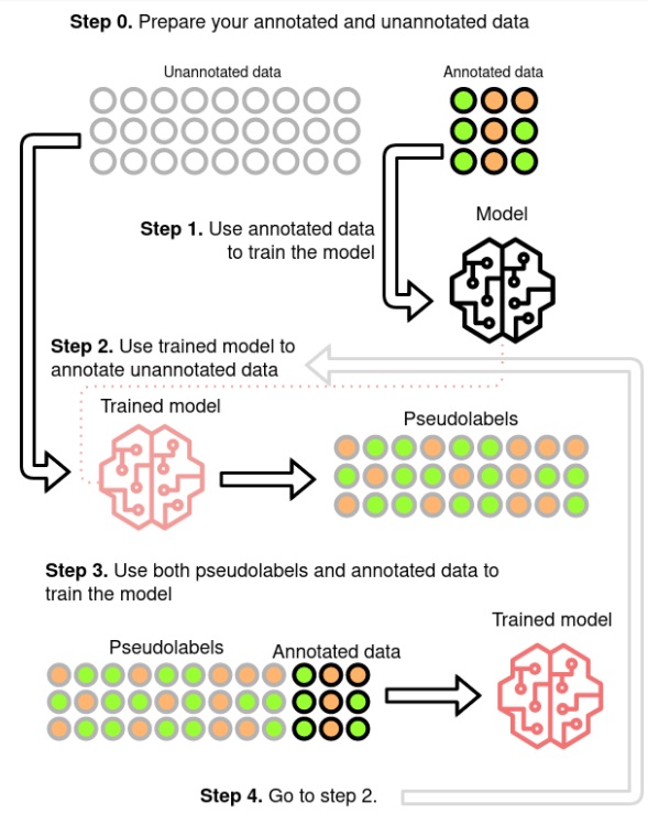
Pseudo-labeling method (source)
Having improved the model in a Pseudo Labelled setup the question that arises is if the model, being learned on the unlabelled data, could create a better pseudo labels for it, than the fully supervised one. This was explored in (link) as Iterative Pseudo Labelling and in (link) as Noisy Student Training. Both state that data augmentation, beam-search decoding with an external Language Model (LM) and balance between the labelled and unlabelled sets are the keys for good performance. (link) uses also filtering mechanism, which probably leads to the better results. In both approaches the beam-search decoding and the external LM are the most problematic components. Beam search, because it is computationally expensive, limiting the number of iterations. External LM, because it is biasing the Acoustic Model (AM) (link). (link) proposes Language-Model-Free IPL (slimIPL) rejecting the beam-search and LM, by using the most probable AM outputs combined with a dynamic cache. Using the dynamic cache enables part of the unlabelled examples to be processed again in a short period with the same pseudo labels and it was shown that this greatly increases the stability of the training, especially for experiments with small labelled sets. The instability is most often caused by model pushing itself into outputting ever less labels. Having generated labels only for a part of the true labels, it is encouraged through learning on them to omit even more. Dynamic cache probably by showing the same example again with more labels than the current model would generate is stopping the model from taking that path. There were proposed alternative approaches to stabilize the training using exponential moving average (EMA) (link, link). One of them was even shown to effectively combine with the dynamic caching.
Most of the articles’ experiments are performed on the Librispeech dataset (link), sometimes adding LibriLight (link) for large scale experiments. The dataset consists of audiobook recordings read by voluntary speakers. This gives often not very high quality audio and lot of accents, but they are single speaker recordings of rather static intonation and speed, containing little emotions and background noises. With current SOTA Speech Recognition models (link) it is possible to achieve 1.9% WER for clean and 3.9% for other test sets without any unsupervised or semi-supervised approaches. This brings doubt if the semi-supervised methods could perform well on real-life data. (link) tests the slimIPL on Conversational Telephone data, but those popular sets (Switchboard (link), Fisher (link, link)) can be classified as single source (single domain). Combining multiple models it is possible to achieve even 5% WER on the corresponding test set, which is not achievable on real-world telephone data (link) (the authors stated on Interspeech 2017 presentation that real-world data had ~20% WER on this model). (link) uses public videos as training data for English and Italian. It is hard to judge the quality of the data, but the semi-supervised approach gives almost same results using only 10h of labelled data and 75kh of unlabelled compared to 650h labelled data in supervised training, which makes the acoustic models creation much faster and cheaper. So it is not exactly clear how the Pseudo Labelling would perform if the labelled data would be of much different acoustic domain than the unlabelled or if the unlabelled would come from lots of acoustic domains.
In our Pseudo Labeling experiments we used modified version of Performance Monitoring (link) to filter out the audio files that are predicted to have worse WER than a threshold. It is working well for high quality audio like data from media. The correlation between predicted WER and real WER is pretty good, but when used for lower quality 8kHz telephone data the WER correlation is not good enough. Experiments with such data show, that the resulting model is performing worse than a model on labeled data only.
Inferring from our experiments and from articles one can state, that the Pseudo Labeling approach is working well if the data is of high quality and the model can predict labels with pretty high accuracy. If the quality of the audio is lower and even the human error is pretty high, the recognitions will give lots of errors, so for some corpora the pseudo-labelled data can bring more harm than good. The second argument against using it for telephone data is the data augmentation. As for SpecAugment it can be accepted that it does not shift the domain of the data, but adding noise could be seen as such shift. So the best way to improve for such data would be augmenting a better quality to an approximation of the telephone quality, but such a domain shift is a separate research area by itself.
In comparison to Self-Supervised learning Pseudo Labelling seems to be less computationally expensive (slimIPL’s 83.2 vs Wav2Vec2.0’s (link) 294.4 GPU-days)(link), but if working on multiple languages probably this would shift on the other side, because of easier reusability of the pre-trained Self-Supervised model. A great news is that the slimIPL can be combined with models like Wav2Vec2.0 and adds additional value on top of them (link, link). As for the multilingual usage a procedure was proposed (link), but compared to Self-Supervised training it is a pretty complex one.
So the Pseudo Labelling approach is best suited if one stays in a relatively closed domain and has lots of real-life data of decent quality. The good thing is that it could be setup in a self-learning mlops manner, that is continuously improving by combining the available labelled data with new incomming production data. This should improve the model both generally, but especially for the new domains that will appear. To enhance the process part of the most difficult filtered-out examples could be sent to the human-in-the-loop and come back as labelled data improving also for the worst quality data.
Share
Author: Jakub Kaliski
Share
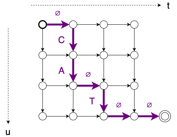
Connectionist Temporal Classification(CTC)(link) is one of the most popular criterion in Speech Recognition. It brings both good performance and training simplicity, but one of main disadvantages is conditional independence of labels. Another one is requirement for input to be longer than output. RNN Transducer (RNNT)(link) was proposed to overcame those issues. New loss function expands CTC mechanisms – blank label and time-restricted alignment, presents some new improvements, and removes inconveniences.
To address first problem, RNNT introduces new model architecture consisting of Predictor Network combined with Encoder Network in Joiner Network.

Encoder behaves as acoustic model – produces latent representation of acoustic features. Predictor consumes sequence of text tokens, thus can be seen as inner Language Model. Joiner sums both modules outputs and proceeds with simple feedforwad layer transforming latent representation to output labels probability distribution. The main idea is to support acoustic part of speech recognition with lexical dependencies built on recognition history. Both Encoder and Predictor network can be transferred from pretrained models – CTC, CE or other tasks, like wav2vec, can be utilized as Encoder while Predictor can be initialized with Neural language Model. RNNT operates in time and labels space, thus allows multiple outputs for single input, which solves second problem.
Incorporating Predictor Network can be beneficial not only in terms of modeling capability. Since Predictor operates purely on text input, it can be easily pretrained on large amount of data. Predictor can also be adapted to new domain using this mechanism (link, link). In contrast to audio, large amount of text data suitable for training are easily available. It also allows to make use of user data, ie on contact list on mobile device. Such single module adaptation can be performed directly on device, assuring privacy.
Unlike standard Attentions models, RNNT can run in streaming fashion, even on mobile devices (link). Seq-2-Seq models tend to relay on full input sequence. It is possible to restrict their inference to current(or contexted) input, but it has impact on performance. In contrary, RNNT itself does not model time dependencies, thus can run in streaming fashion out of the box. Forcing Seq-2-Seq models may also bring noticeable delay into system. RNNT model latency can be controlled in multiple ways – with loss function restrictions utilizing alignments (link) or forcing monotonic outputs, decoding strategies (link) or auxiliary losses (link). RNNT seems to work well with wordpieces outputs (link, link), which helps to keep good realtime and computational complexity by reducing output steps number.
With all this features come some drawbacks. The most severe one is training memory consumption. Since acoustic and text representation can vastly differ in length, they cannot be simply added. We can combine two 3D matrices using broadcasting, but it forces huge memory overhead due to spare paddings (link). Keep in mind it’s only forward pass, we need to keep parameters for backpropagation as well. Alongside common ways of reducing memory footprint, like using half precision or training using examples sorted by length, some new techniques were proposed. Broadcasting was replaced with per utterance combination (link) followed by concatenation, so there is no extra padding added to shorter examples. The same article utilizes merging softmax function into loss computation, which can save extra memory when using large amount of wordpieces. Recently k2 project team put their effort to optimize RNNT memory footprint. They implement some of already proposed solutions (Recurrent Neural Aligner – restricted varaint of RNNT so it can emit only one symbol per frame), as well as some new ideas, like pruned RNNT. This approach minimizes memory usage by pruning zero gradients from backproagation.
Also predictor can introduce some exposure bias to model – training on small amount of data may lead to overfitting and generalization issues. Some methods to prevent this aim directly at training procedure (link), while other propose architecture changes (link) or training pipeline tricks (link). With all mentioned above, RNNT models can be challenging to train and diagnose.
Despite problems, RNNT seems to gain more and more attention, and list of frameworks offering RNNT keeps growing. Here are some of them:
NeMo (link)
SpeechBrain (link)
PyTorch (link)
k2 (link)
ESPnet (link)
There are some standalone implementations offering bindings to popular libraries like PyTorch or Tensorflow (link). Surprisingly, there is no official implementation in Tensorflow, despite Google seems to put some effort in RNNT development (link). Efficient RNNT implementations from k2 are available as separate modules (link).
Combining all together, we think RNNT can lead to further speech recognition improvements. Incorporating lingual aspect directly into acoustic model may boost generalizing abilities, especially in challenging acoustic conditions. Predictor adaptation using only text data may be easy way dealing with new/out of domain data. Keep in mind, that so far we only considered ASR systems without external Language Model. While in conventional systems, Language Model integration is quite straightforward, RNNT offers few strategies of fusion, like deep, shallow or cold. (link)
It seems that RNNT can lead to SOTA results in some products, like mobile devices systems or streaming applications. Modular design allows to use pretrained Encoder and Predictor networks as single pipeline in end-to-end manner and greatly simplify speech recognition system. With more attention from research teams, RNNT will improve in field of memory footprint, training stability and overall performance.
Share
Author: Jakub Filipiuk
Share

Share
Authors: Piotr Pęzik (UŁ/VoiceLab), Agnieszka Mikołajczyk, Adam Wawrzyński (VoiceLab), Bartłomiej Nitoń, Maciej Ogrodniczuk (IPI PAN)
Share
Self-supervised pre-training is one of the most promising methods in the deep learning field. Following Computer Vision and Natural Language Processing, it recently became one of the most popular topics in Automatic Speech Recognition (ASR) research. The proposed Contrastive Predictive Coding (CPC) (link) has shown great potential in using unlabeled data for Phone and Speaker Classification. This has now marked the start of a huge effort led by the big tech companies to utilize the most out of the ocean of unlabeled speech data that is currently available on the Internet.
The reason why this is such an appealing topic is due to the large financial cost of labeling large amounts of speech recognition data for use in the training of Speech Recognition Systems. Current commercial ASR corpora can cost up to a few hundred dollars per hour of data. Examples include the American English Speech Recognition Corpus (Mobile) from ELRA (link), which costs 6000€ for 14.67 hours of speech. Combined with the observation that in order to reduce the Word Error Rate (WER) by 50% for a neural network model (link) the dataset must increase by a factor of 10, we come to the conclusion that it is only feasible to do achieve a certain WER, after which the returns are diminished by the financial cost of buying or labeling new data. Furthermore, achieving a satisfactory WER via datasets of transcribed audio is only practical for the most commonly spoken languages, where the client base is much greater. For this reason, big tech companies and the rest of the industry have been focused on finding different, more scalable solutions.
Since the original CPC article and its extension wav2vec (link), which was the first to show its ability to achieve comparable state-of-the-art (SOTA) results on a commonly used dataset, there has been a wave of articles and research further adding and expanding upon the original work, combining it with some existing research or simply using it for other tasks or domains. The most important work uses wav2vec2.0 (link), which beat the SOTA results on the LibriSpeech (labelled) + LibriLight (unlabeled) datasets. This was achieved by using another promising method: Noisy Student Training (link), also known as Pseudo Labelling (link), which we will cover in a separate post soon. The best feature of the two methods is the fact that they can be successfully combined (link, link), with the main drawback of the wav2vec2.0 versus CPC or wav2vec being that it uses a large full context Transformer model and a masked based training procedure, so it cannot be used in a low-latency ASR system.
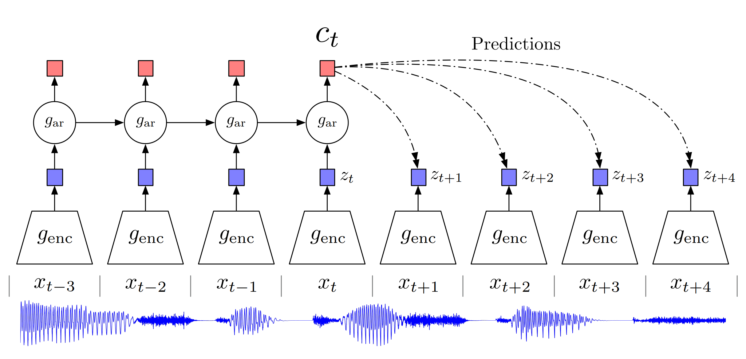
Overview of Contrastive Predictive Coding, the proposed representation learning approach.
Although this figure shows audio as input, we use the same setup for images, text and reinforcement learning. (source)
The main idea in self-supervised learning is to learn some kind of representation of the input signal that can be useful for the downstream task. To do so, we need to define a loss function that can learn something meaningful. Both the original CPC and wav2vec2.0 losses are inspired by the losses used in language modelling. The Recurrent Neural Network Language Models (link) were trained to predict the next word having the current word as input and all previous words as context. This paradigm forces the neural network to learn a representation of each word and their combination to be able to predict which next words are making sense in this context, thus learning the structure of a language purely by receiving lots of text data, which is very easy to attain in large quantities. Having such a pre-trained model, one can fine-tune it to a more precise task where the data is much sparser, such as Text Classification (link). The same goes for CPC, but due to the unclear boundaries of a speech signal, its variability and sample density (usually 8k or 16k per second), a latent signal representation is needed to make the prediction task a reasonable one. This introduces the problem a new problem to the model, wherein it may simply “collapse” by zeroing out the latent representation and achieving a 100% accuracy rate. To prevent this, the contrastive task was proposed: to distinguish following frames from N randomly sampled ones, which forces the representations to differ. As the speech signal can stay longer in some phonemes than in others, in order to give more incentive to learn, the model is set to predict more than one succeeding latent representations, preventing it from making a simple prediction that the latent vector will always stay the same because it should be true for a significant portion of the time. Combining this has given the authors a method to successfully train a model which achieved promising results on both Phone and Speaker Classification tasks. The following wav2vec proved that it is useful as pre-training of Acoustic Models (AM) for ASR.
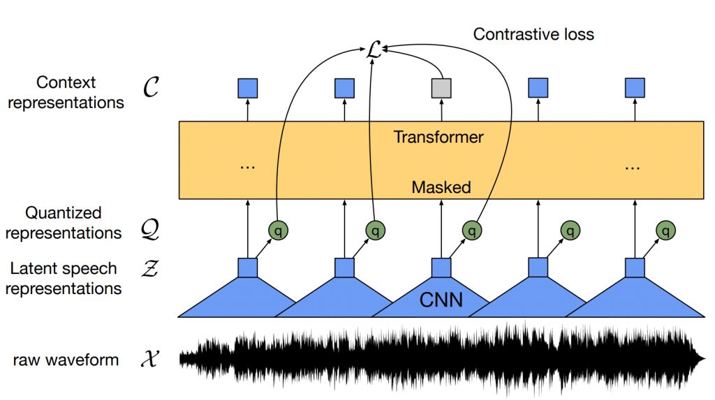
Illustration of framework which jointly learns contextualized speech representations
and an inventory of discretized speech units. (source)
The wav2vec2.0 was inspired by the BERT model (link), where having a model that needs a full future context the prediction of the next token was infeasible. To mitigate this, Masked Language Modeling (MLM) was proposed where some input tokens are masked and the model has to predict them. In wav2vec2.0 the model is trained in the MLM fashion, but on the quantized latent representations. This forces the use of contrastive loss, Gumbel SoftMax (link), and a diversity loss (link) to encourage the usage of all classes. The use of powerful Transformers and MLM-like procedures has enabled valuable pre-training and reduced the need for labelled data, giving great results also for other languages that were not included in the pre-training (link). Further research tries to add something on top of this, such as offline clustering of similar frames to discover hidden units in HUBERT (link), additional loss functions (link, link), which brings some small gains or more robustness in some domains or simply scaling (link). The big problem in these models is the cost of the pre-training, which for the original wav2vec2.0 was around 16000 GPU-hours [5], as well as its instability (link, link). So taking all data you can get and throwing it into the model is not the best idea. Besides, although the models are great for in-domain data, when faced with some domains that are further apart from the data used in pre-training it does not so well (link). The proposed remedy is to do a pre-training continuation on the target domain data, which gives large WER reduction even if the fine-tuning data is not in the target domain, but still requires a lot of the unlabeled target data to really make a difference. So, in terms of generalization, the speech community still has much to discover, even outside the pure self-supervised training domain (link).
Self-supervised pre-training is a great effort to make speech recognition more available for the less spoken languages, especially due to the openness of the big companies and the machine learning community, which provide models with their research. If this were not the case, pre-training such models would be unachievable for most researchers and small companies due to the enormous GPU computational cost. Still, moving outside of the target domains brings lots of challenges in and of itself. Furthermore, as the research progresses into ever larger models (link) we will soon face Megatron-Turing NLG-like (link, link) sizes, which will only be attainable for companies with large financial means. In summary, despite the fact that hardware is improving by great leaps and bounds, what most needs improvement are the methods used to train such enormous models, preferably to reduce them to only a fraction of the computational cost that they have today. Hopefully, some breakthroughs in this matter will be coming soon.
Share
Author: Jakub Kaliski
Share
What do you think, when you hear ‘Transformer’? Is it a robot? A component used in an electrical circuit? Or maybe a neural network? If you want to find out something about the last one, welcome to read it!
Transformers are the family of neural networks mainly used in Natural Language Processing (NLP) and were introduced relatively recently – in 2017 by Vaswani et al., in the paper “Attention Is All You Need” (link). A fancy title indeed communicates the main idea of the architecture.
Previously, in NLP there were mostly used recurrent neural networks (RNN). Although having satisfying results, they had a drawback of computation time, as they consider a long sequence of words at a time. Here, as a rescue come transformers because they don’t operate on the whole sequence but only on the attention relationships between embeddings (numerical representation of words).
Previous architectures were based on the encoder-decoder structure. The encoder had to create a vector representing the input sentence and then passed as an input to the decoder.
Attention mechanism assumes passing all the encoder states to the decoder so that the model can choose which information it considers as most important.
In figure 1 you can see the idea of the attention mechanism in the translation process. Although the idea might seem simple, it was a breakthrough in the field of natural language processing.
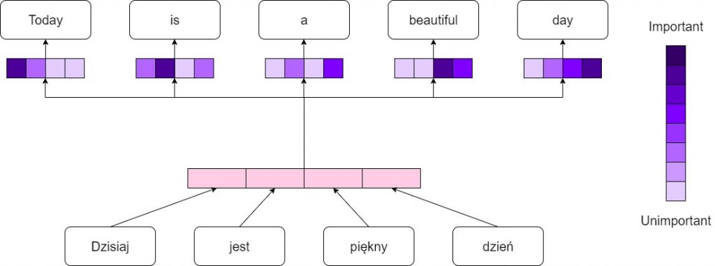
Attention mechanism
When we consider a self-attention mechanism the difference is that the choice of which part of the input is the most important is made during the encoding process – inputs interact with each other scoring with the “attention points”.
As you can see in figure 2, the encoder consists of n layers with two sub-layers inside each of them. One is a Multi-Head Attention that independently learns the self-attention between words and the second one is a fully connected feed-forward network. The sublayers are joined together by the residual connections followed by the normalization block.
The Transformer architecture
The decoder has a pretty similar structure, however, each layer has additionally a third sub-layer, which is a Multi-Head Attention over the output of the encoder.
The Multi-Head Attention mechanism is performed on three vectors – Query, Key and Value. The query may be considered as a current word (embedding), while value is the information it carries. A key is just a form of order of values, like indexing.
Transformers allow for text analysis from a different perspective – not as a sequence of words, but rather the gist of the message. It’s a huge advantage as normally the order of words in the sentence differs depending on the language, speaker, etc. Although Transformers are more efficient in terms of computation, they need a huge amount of data to be trained which is a common problem regarding machine-learning issues.
Fortunately, there are models that might be used as a base for transfer learning like e.g. HerBERT (link). This model was introduced in 2021 by polish scientists from Allegro.pl. It is based on the BERT – the most known model for NLP created by Google and adjusted to the difficult polish language. In the KLEJ classification, it managed to reach 88,4 out of 100 points which is the state of the art result regarding polish models.
To use the model you can simply put it like this:
from transformers import AutoTokenizer, AutoModel

tokenizer = AutoTokenizer.from_pretrained("allegro/herbert-base-cased")
model = AutoModel.from_pretrained("allegro/herbert-base-cased")

output = model(
    **tokenizer.batch_encode_plus(
        [
            (
                "Język – ukształtowany społecznie system budowania wypowiedzi, używany w procesie komunikacji.",
                "Język służy do przedstawiania rzeczywistości dotyczącej przedmiotów, czynności czy abstrakcyjnych pojęć za pomocą znaków.",
            )
        ],
    padding='longest',
    add_special_tokens=True,
    return_tensors='pt'
    )
)
In this case, you have to define a tokenizer – a tool to divide input into separate tokens – words and a model that you want to use – i.e. herbert-base-cased. As an input to the model, you put a tokenized text.
Depending on what you want to do, you can use HerBERT with an appropriate Head Model for different purposes, i.e.:
Predicting a masked word in the sentence,
Predicting the next word,
Predicting the next sentence,
Answering questions
As an output, you get a desired word or sequence of words.
Computer Vision is one of the fields where machine learning is gaining the most interest. Most of the solutions apply to vision problems. Even analysis of a signal is sometimes transformed to an ‘image form’ and then processed by a network. If so, why not give it a try for a reverse operation?
The usage of Transformer in image recognition was introduced in the paper “An Image is Worth 16×16 Words: Transformers for Image Recognition at Scale” (link) in 2020 by Dosovitskiy et al.
The main idea was to divide an image into smaller patches of the same shape. Let’s imagine, that each of these patches is a ‘word’. Next, we have to vectorize them. This means, putting all the values from one patch into a vector with a given order. From each vector x then are created functions z with parameters W and b which are the parameters of the network learned in the training process. Additionally, there is added information about positional encoding. It is important to keep the correct order of the patches. Then the Multi-Head Self-Attention layer comes and the magic happens, as in the original Transformer.
As you can see in figure 3, the whole model does not vary much. It’s the input preparation that has to be different than in the original transformer.
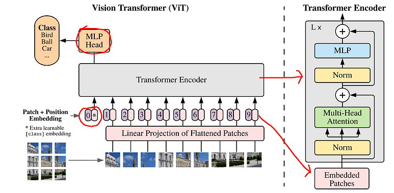
Vision Transformer architecture
To use the Vision Transformer model you can use a timm library:
import timm
import PIL
import torchvision.transforms as T

model_name = "vit_base_patch16_224"
model = timm.create_model(model_name, pretrained=True)

IMG_SIZE = (224, 224)
NORMALIZE_MEAN = (0.5, 0.5, 0.5)
NORMALIZE_STD = (0.5, 0.5, 0.5)
transforms = [
              T.Resize(IMG_SIZE),
              T.ToTensor(),
              T.Normalize(NORMALIZE_MEAN, NORMALIZE_STD),
              ]

img = PIL.Image.open('samochod.jpg')
img_tensor = transforms(img).unsqueeze(0)

output = model(img_tensor)
You can define a model from the library. It’s an already pre-trained model, ready to use. As an input, you provide an image as a tensor – a common type of data used in computer vision. As an output, you get a class to which the object belongs and a score of confidence. It’s important that you don’t have to do all the input preprocessing manually, this is done for you 😊
Both Transformer and Vision Transformer are based on the same idea – attention. As long as the model engine is the same in both of them, a distinct difference is visible in the input and output. A standard form of providing text into the model is tokenization. The image has to be transferred to a similar form – cut into small pieces and put in order. The output also differs as the aim of the task is different. When providing text, we want to “explore the unknown” – see something that we do not know yet, while during the image processing we rather want to analyze what is visible in it.
Most of the commonly used models in NLP are based on the Transformer. Mostly, they are used in bots as a form of communication with the customer.
When it comes to Vision Transformers, they gain popularity among other great models. They can be used in image classification, detection or segmentation, for example in medical image analysis.
As every model, Transformers have their pros and cons. Training a valuable transformer from scratch is extremely hard – huge amounts of data and computational power are needed. However, usage of already existing ones gives an opportunity to benefit from their ability to “read the context”. Considering various problems – context is rather more important than details.
To sum up – Attention is all you need! 😊
Share
Author: Maria Ferlin, Politechnika Gdańska
Resources:
Share
Without a doubt, COVID-19 has had a great impact on today’s world. It has changed nearly all aspects of daily life and has become part and parcel of social discussion. Due to many COVID-19 restrictions, the majority of conversations have moved to social media, especially to Twitter which is one of the biggest social media platforms in the world. Since the opinions posted there highly influence society’s attitude towards COVID-19, it is important to understand Twitter users’ perspectives on the global pandemic. Unfortunately, the number of tweets posted on the Internet is enormous, thus an analysis performed by humans is impossible. Thankfully, for this purpose, one of the fundamental tasks in Natural Language Processing – sentiment analysis – can be performed which classifies text data into i.e. 3 categories (negative, neutral, positive).
Today, we would like to share with you some key insights on how we performed such sentiment analysis based on scraped Polish tweets related to COVID-19.
In the beginning, we had to scrape the relevant tweets from Twitter.
Since we were particularly interested in analyzing the pandemic situation in Poland, we downloaded tweets which:
were written in Polish,
were posted from the beginning of the pandemic (March 2020) until the beginning of the holidays (July 2021),
contain at least one word from the empirically created list of COVID-19 related keywords (such as “covid” or “vaccination” etc.)
With the following approach, we successfully managed to scrape more than 2 million tweets with their contents and variety of metadata such as:
the number of likes under a given tweet,
the number of replies under a given tweet,
the number of shares of a given tweet, etc.
However, for the purpose of training the model, we also had to obtain data with the previously labeled sentiment (negative, neutral, positive).
Unfortunately, there is currently no dataset that is publicly available containing Polish tweets about COVID-19. That is why we had to extend the publicly available Twitter dataset from CLARIN.SI repository with 100 personally labeled COVID-19 tweets in order to train a model on a sample of domain-specific texts.
Before starting the training process, the data preprocessing step was performed. It was especially important in our case since the Twitter data contains a lot of messy text such as reserved Twitter words (eg. RT – for retweets) and users’ mentions. With the use of the tweet-preprocessor library, we removed all of these unnecessary text parts that could become noise for a model.
Moreover, we replaced the links with the special token $URL$ so that each link is perceived by the model as the same one. It was particularly important since in the later phase we noticed that the information of link presence is valuable for the model predictions.
At the end of the preprocessing stage, we decided to replace the emoticons with their real meaning (eg. “:)” was changed to “happy” and “:(” was replaced by “sad” etc.).
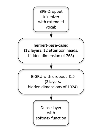
Having cleaned the data, we were able to build a model. We decided to base it on HerBERT (Polish version of BERT) since it receives state-of-the-art results in the area of text classification. We followed it with two layers of a bidirectional gated recurrent unit and a fully connected layer.
The BPE-Dropout tokenizer from HerBERT (which changes a text into tokens before passing input to HerBERT) was extended with additional COVID-19 tokens so that it would recognize (not separate) the basic coronavirus words.
| Metric | Score |
| F1-Score | 70.51% |
| Accuracy | 72.14% |
| Precision | 70.60% |
| Recall | 70.44% |
The model receives relatively good results even though Twitter data is often considered ambiguous when it comes to the sentiment label itself and ironic.
With the trained model, the sentiment for previously scraped COVID-19 tweets was predicted. This allowed us to perform a more detailed analysis, which was based not only on collected metadata (eg. likes, replies, retweets) but also on predicted sentiment.
When the weekly number of tweets for each sentiment is visualized over time, some negative “picks” can be observed
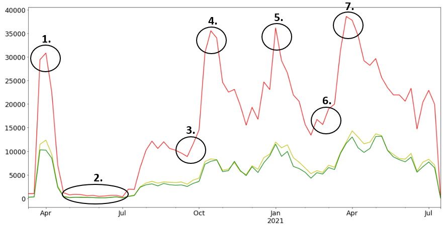
In the majority of cases, they are strictly correlated with important events/decisions in Poland such as:
Postponement of the presidential election
Presidential campaign
The beginning of the second wave of COVID-19
The return of hard lockdown restrictions
The beginning of vaccination in Poland
The beginning of the third wave of COVID-19
The daily record of infections (over 35,000 new cases)
When we decided to dive deeper into the content of negative Tweets, these were the most frequently used negative expressions:
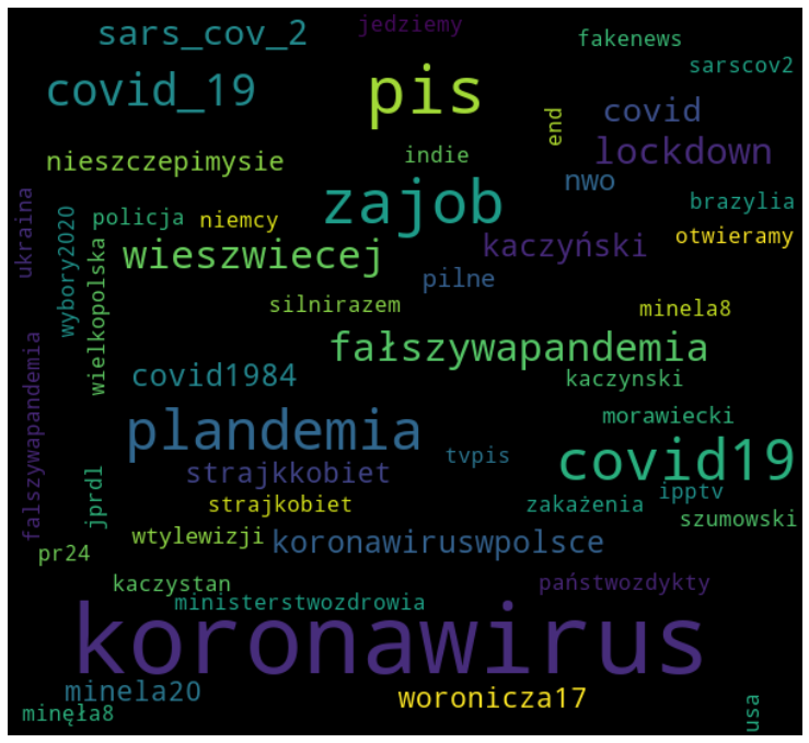
Undoubtedly, they are slightly biased towards the keywords based on which we scraped the Tweets, but overall they give a good sense of topics covered in negative tweets i.e. politics and popular tags used in fake news activities.
Moreover, we were interested in analyzing who is the most frequently tagged account in these negative tweets. It came out that:
most frequently the politicians are blamed for their pandemic decisions
the accounts of the most popular television programs in Poland are a big part of COVID-19 discussions
Last but not least, we decided to analyze the Twitter accounts that influence society the most with their negative tweets (those that gain relatively the most likes/replies/retweets).
Unsurprisingly, these are politicians from the Polish opposition who are present at the top of the list.
To sum up, as we can all see, sentiment analysis accompanied by data analysis can give us interesting insight into the study community’s characteristics. It brings a lot of benefits and allows us to utilize huge amounts of text data effectively.
Share
Authors: Michał Laskowski, Filip Żarnecki
Share
A way to grasp what your NLP model is trying to communicate.
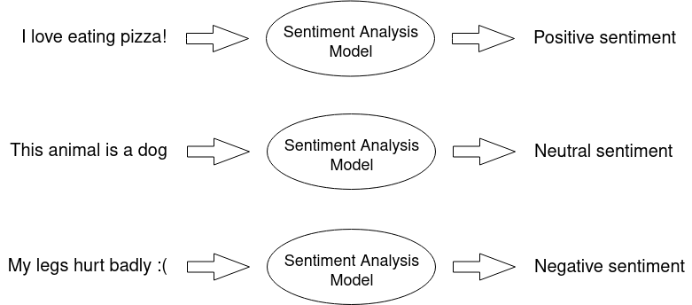
Sentiment Analysis is basically a recognition of an utterance’s emotional tone – in our case, the AI solution tells us whether given statement is negative, neutral or positive:
We have already described our approach, data used, processing of data and model architecture in more detail in a previous article. In short, we use a solution based on HerBERT and train it using labeled Twitter data.
We have decided to make use of XAI (explainable AI) in order to better understand our model’s decision-making. We wanted to see which features influence the final verdict the most and whether we can identify some room for improvement.
XAI (eXplainable AI) is an AI concept that enables us, humans, to understand predicted results better. We open the black box, you could say.

Most of us have heard of the term ‘black box’ when referring to Deep learning models. It is defined as a complex system or device whose internal workings are hidden or not readily understood. It has originated from the fact that usually even model developers cannot state why the AI has come to a specific conclusion.
On the one hand, some might say it is beneficial to develop deep, multilayered models without needing to understand the whole decision process, and they are not wrong. It takes away worries and makes the process somewhat convenient. However, how can we be so sure that our prediction is based on good premises?
Even if we achieve high accuracy scores on the test set, it might not be the real-world inference accuracy. The results will also be biased if the dataset is biased, and high-performance results mislead us to believe that the system is just fine. Models’ robustness is especially important in domains like medicine, finance, or law, where it is crucial to understand the reasoning behind a decision when its consequence might be fatal.
It can be highly beneficial to try and dig deeper into the unknown of mentioned above ‘black box’. The inability to fully explain AI decision-making has been quite troublesome over the years.
There is a phenomenon that can, in short, be described as Algorithm aversion – a situation where people lack trust in algorithmic model decisions, even knowing that it outperforms human beings.
People fear what they do not understand, and this is usually the case with the black box models. The inability to grasp why the AI model has decided one thing instead of another causes insecurity and doubts. In turn, that leads to a lack of trust and decision rejection that could be better than our judgment.
It is logical to assume that people would be more likely to listen to AI if they better understood the decision-making process.
We can distinguish two main types of approaches to explaining the model predictions:
building a simpler, transparent model
sing a black-box model and explaining it afterwards
Transparent ML models, such as a simpler decision tree, Bayesian models or linear regression, even though easily interpretable, have often proven to be outperformed by their black-box friends. Therefore, since we want the best performance possible, we need the additional post-hoc layer on top of our solution.
Post-Hoc meaning after the event, in our case, means an explanation done after making a prediction (or series of predictions).
Explanations can be Model Agnostic (works with any model) or Model Specific. The one that interests us the most is the Model Agnostic since it will explain any model, regardless of the architecture.
We also want to focus on the idea of the Feature Importance – to measure how an individual feature (input variable) contributes to the predicted output.
Such an approach very neatly suits the Natural Language Processing (NLP) domain.
In NLP classification problems, we are often supposed to analyze a sequence of words provided as an input and get the probability of each class affiliation as an output.
Basically, when explaining a single prediction, we want to measure how each element of an input contributes to each class probability. It’s pretty straightforward. The difficulty now is how to do it.
Over the past years, many algorithms have been developed. Here, we chose two Explainers based on their simplicity and understandability: LIME and SHAP. The solutions we use are rather intuitive and easy to grasp.
LIME is one of the first perturbation-based approaches to explaining a single prediction. As we can read on projects github page:
Lime can explain any black-box classifier with two or more classes. All we require is that the classifier implements a function that takes in raw text or a NumPy array and outputs a probability for each class.
As a result, we can apply LIME to any model that takes in raw text or a NumPy array and provides a probability for each class as an output.
But what does it do exactly?
The main idea is that it is easier to approximate the whole model with a simpler local model. How can that be achieved?
We perform a perturbation of the input sequence (e.g. we hide one sentence word (marked with MASK token)) and check how the predictions differ. Then the perturbed outputs are weighted by their similarity to the explained example.
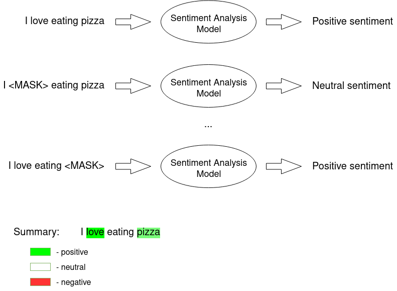
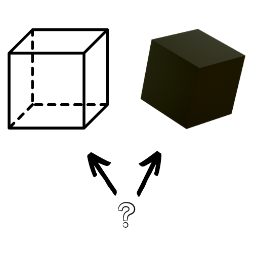
Intuitively, an explanation is a local linear approximation of the model’s behavior. While the model may be very complex globally, it is easier to approximate it around the vicinity of a particular instance. While treating the model as a black box, we perturb the sample we want to explain and learn a sparse linear model around it as an explanation. The figure below illustrates the intuition for this procedure. The model’s decision function is represented by the blue/pink background and is clearly nonlinear. The bright red cross is the instance being explained (let’s call it X). We sample instances around X and weigh them according to their proximity to X (weight here is indicated by size). We then learn a linear model (dashed line) that approximates the model well in the vicinity of X, but not necessarily globally.
Since the input is in the form of understandable words, we can then easily interpret the provided results. On the output, we receive a list of all features and their contribution to each of the classes.
Exemplary visualisation:
We can see in the image above how different features (words) contributed to each class. E.g. ‘boli’ caused the probability of the ‘negative’ class to rise and lowered the likelihood of the ‘neutral’ class.
This algorithm is somewhat similar to the LIME as it also perturbs input to make explanation. However, in a bit different way.
If you would like to understand all the details behind SHAP methodology, here is a great article that talks about the subject in a really understandable manner.
In short, SHAP is a calculating contribution that each feature brings to the model prediction. The contribution is based on the idea that in order to determine the importance of a single feature, all possible combinations of features should be considered (a power set in maths). Therefore, SHAP approximates all the possible models from the provided dataset (i.e., the input we have provided in a given explanation). Having all possible combinations, all of the marginal contributions are taken into account for each feature.
Marginal contribution of a certain feature is a situation where there are two almost exactly the same scenarios with the only difference being a presence (or absence) of our feature of interest.
All the marginal contributions are then aggregated through a weighted average, and the outcome represents contribution of a given feature to a given class. The summary can then be visualised, e.g. with a force plot, such as the one below:
Here, the features that increase the probability for a given class are highlighted with red and those that lower it with blue. The base value is the average model output over the training dataset we have passed.
Having our algorithms selected and explained, we can see how they perform in practice. In our case, during the analysis of Polish utterance emotional tone.
To recap, we are using model based on HerBERT (Polish BERT), and we have distinguished three classes – negative, neutral, and positive.
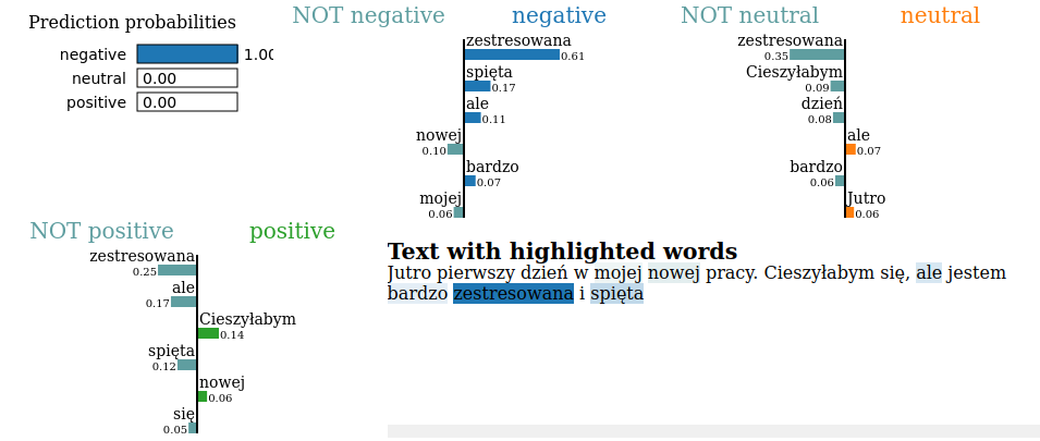
Exemplary utterance to analyse:
Jutro pierwszy dzień w mojej nowej pracy. Cieszyłabym się, ale jestem bardzo zestresowana i spięta
True sentiment: negative
Predicted sentiment: negative
As we can see, the model has correctly predicted negative sentiment within the provided sentence, even though the example is a little tricky. Now, let’s move on to the explaining process and check which features influenced this decision.
Firstly, let LIME show its performance. We load our model from a checkpoint:
device = 'cpu'
        model = HerbertSentiment.load_from_checkpoint(model_path,
                                                        test_dataloader = None,
                                                        output_size = 3,
                                                        hidden_dim = 1024,
                                                        n_layers = 2,
                                                        bidirectional = True,
                                                        dropout = 0.5,
                                                        herbert_training = True,
                                                        lr = 1e-5,
                                                        training_step_size = 2,
                                                        gamma = 0.9,
                                                        device = device,
                                                        logger = None,
                                                        explaining = True)
Then we setup the LIME:
tokenizer_path = "allegro/herbert-base-cased"
        tokenizer = AutoTokenizer.from_pretrained(tokenizer_path)
        target_names = ['negative', 'neutral', 'positive']

        explainer = LimeTextExplainer(class_names=['negative', 'neutral', 'positive'])
Finally, we make the explanation.
input = "Jutro pierwszy dzień w mojej nowej pracy. Cieszyłabym się, ale jestem bardzo zestresowana i spięta"

        explanation = explainer.explain_instance(input, model.forward, num_features=6, labels=[0,1,2])
… and print the results:
print ('Explanation for class %s' % target_names[0])
        print ('\n'.join(map(str, exp.as_list(label=0))))
        print()
        print ('Explanation for class %s' % target_names[1])
        print ('\n'.join(map(str, exp.as_list(label=1))))
        print()
        print ('Explanation for class %s' % target_names[2])
        print ('\n'.join(map(str, exp.as_list(label=2))))
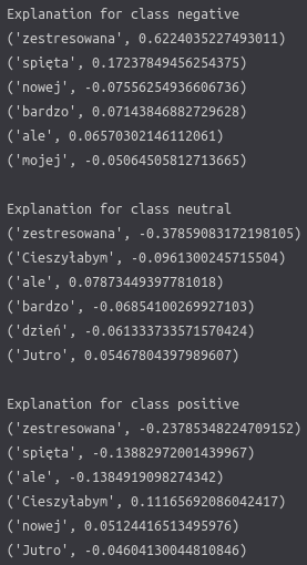
Those messy numbers in the picture define how a certain word influenced each of the classes. If a number is >0 then it increased the chance for the class. On the contrary, if it is <0 it decreased it.
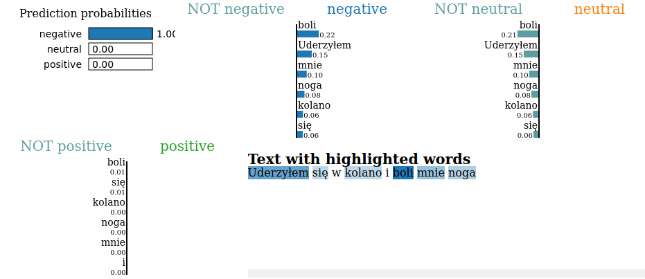
explanation.show_in_notebook()
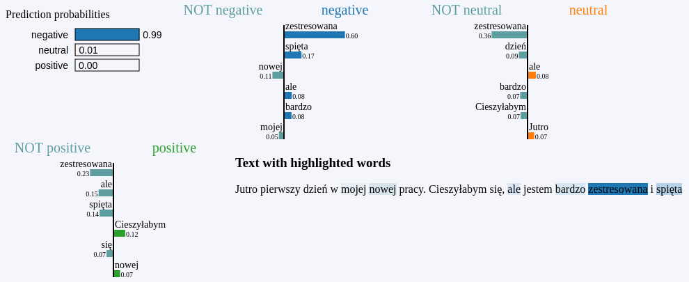
In the dedicated LIME visualisation above, it is a bit easier to interpret the results. We can quickly tell which tokens were the most influential for which class. For example, the word ‘zestresowana’ significantly impacted all categories, greatly increasing the chance for negative and reduces bothneutral and positive ones.
As you can see, it can provide some helpful insight.
Now, let’s compare all this to SHAP…
We load the model in the same manner:
device = 'cpu'
        model = HerbertSentiment.load_from_checkpoint(model_path,
                                                        test_dataloader = None,
                                                        output_size = 3,
                                                        hidden_dim = 1024,
                                                        n_layers = 2,
                                                        bidirectional = True,
                                                        dropout = 0.5,
                                                        herbert_training = True,
                                                        lr = 1e-5,
                                                        training_step_size = 2,
                                                        gamma = 0.9,
                                                        device = device,
                                                        logger = None,
                                                        explaining = True)
Then we set up the SHAP:
tokenizer_path = "allegro/herbert-base-cased"
        tokenizer = AutoTokenizer.from_pretrained(tokenizer_path)
        target_names = ['negative', 'neutral', 'positive']

        explainer = shap.Explainer(model, tokenizer)
Prepare methods for the results visualization:
def print_explanation(shap_values):
            values = shap_values.values
            data = shap_values.data
            for word, shap_value in zip(data[0], values[0]):
                print(word, shap_value, '---', target_names[np.argmax(shap_value)])

        def print_contribution(shap_values):
            print('\n')
            print("Contribution to negative class")
            shap.plots.text(shap_values[0, :, 0])
            print('\n')
            print("Contribution to neutral class")
            shap.plots.text(shap_values[0, :, 1])
            print('\n')
            print("Contribution to positive class")
            shap.plots.text(shap_values[0, :, 2])
Finally, we make the explanation…
input_to_explain = ["Jutro pierwszy dzień w mojej nowej pracy. Cieszyłabym się, ale jestem bardzo zestresowana i spięta"]

        shap_values = explainer(input_to_explain)
… and print the results:
print_explanation(shap_values)
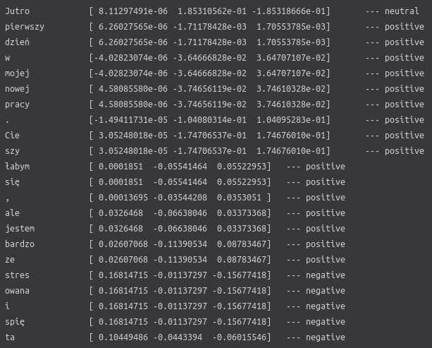
We can see numbers that show how sentence tokens contribute to each class, much like they do in LIME. Additionally, there is a dominating sentiment shown on the right.
You can notice that some words are divided and analyzed strangely since SHAP is using the HerBERT tokenizer for the explanation process. The tokenizer analyses the input sequence and looks for each of the tokens (words) in its dictionary. If a particular word does not exist there, it is divided into parts that do. E.g. ‘Uwielbiam’ will be divided into ‘Uwielbi’ and ‘am’. This process helps to ignore possible flection noise resulting from Polish grammar rules (a male variant of a word will differ from a female variant of the same word).
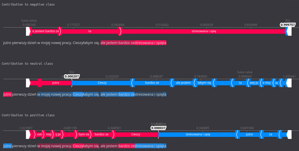
print_contribution(shap_values)

In this more colorful visualization, the same data is presented but in a more comprehensible manner. There is a force plot for each of the classes, along with all of the words contributing. Those marked with red color increased probability for a given class, and those in blue decreased it. We can easily see which tokens were the most influential, both on the force plot and in the highlights in the sentence below the plot.
For instance, we observe that the words (or their parts) ’zestresowana i spięta’ influence the negative sentiment quite a bit while lowering the positive one significantly.
Proper interpretation of such visualisations can give us a good idea of how our model thinks and influences the result the most.
As you can see, XAI provides us with some interesting and valuable insight into our model. The explanation process is not as complex as it might seem, and it is worth the burden considering the benefits. Proper interpretation of the results, including the understandable visualizations, can give us a good idea of how our model ‘thinks’ and what influences the predictions the most.
If your machine learning problem regards one of the domains where algorithm trust is crucial to be developed and where algorithm aversion might cause you a headache, explainable AI comes to the rescue. Keep this in mind the next time you want to dig deeper into your algorithm.
Share
Authors: Filip Żarnecki, Michał Laskowski
Share
In recent years, deep learning-based Text-To-Speech systems outperformed other approaches in terms of speech quality and naturalness. In 2017, Google proposed the Tacotron2 end-to-end system capable of generating high-quality speech approaching the human voice. Since then, deep learning synthesizers have become a hot topic. Many researchers and companies have published their Tacotron2 based end-to-end TTS architectures like FastPitch and HifiGan.
Besides the ongoing research about few-shot TTS models, top architectures still require relatively large datasets to train. Moreover, both spectrogram generators and vocoders are sensitive to errors and imperfections of the training data.
There are datasets within the public domain, such as LJSpeech and M-AILABS. However, only a few of them provide good enough quality, especially in languages other than English.
In this article, we will present our approach to building a custom dataset designed for a deep learning-based text-to-speech model. We will explain our methodology and provide tips on how to ensure high-quality of both transcriptions and audio.
We split it into two parts. The first one will focus on the text and provide data on where to get and how to prepare transcriptions for recording. The second part will mainly cover recording and audio processing.
Keep in mind that there are differences between languages. Some of our findings might not apply to all of them.
First things first, we need to have a source of our text data. The easiest to get and probably the most commonly used sources of text are open domain books.
While we agree that they’re a great source, there are few things to consider:
Many public domain books are old, which might cause transcriptions to be archaic, especially in languages that changed over the years.
They may be lacking difficult words and have little variety (e.g. children’s books).
They might have insufficient punctuation (e.g. there are very few questions in nature books).
Since TTS models learn to map n-grams to sounds, if the dataset lacks some of them (which might be caused by 1 or 2), the model will have problems with their pronunciation. It will be especially noticeable in words with difficult or unique pronunciation (this is often called phoneme coverage). The third might cause problems like not stressing questions or strange behaviour when facedSchodowski with a lot of punctuation – e.g. when enumerating.
Therefore, to ensure good phoneme coverage and a sufficient amount of punctuation, we recommend diversifying the sources of transcriptions.
Each source and genre has its characteristics that we should consider when building a dataset. For example, interviews on average have significantly more questions than news outlets or articles about nature do. Dialogue-heavy stories have more interpunction. Scientific papers will more often have an advanced vocabulary. The press will probably require more normalization (more on that later), some sources might have a lot of foreign words (which we want to avoid), and so on.
If we intend to use our TTS model for something more specific, adding transcriptions that have domain-specific words may also improve the result.
How can we find out how many hours of data we will have from collected text? For that we will need speech rate. Speech rate is the number of words spoken in 1 minute, and the average speech rates are relative to context and language.
Presentations: between 100 – 150 wpm for a comfortable pace
Conversational: between 120 – 150 wpm
Audiobooks: between 150 – 160 wpm, which is the upper range for people to comfortably hear and vocalise words
Radio hosts and podcasters: between 150 – 160 wpm
Auctioneers: can speak at about 250 wpm
Commentators: between 250- 400 wpm
Source
As you can see, the best speech rate for the general use TTS system is around 150 words per minute. The LJSpeech speech rate is approx. 140 wpm. Of course, you should consider your speakers’ natural speech rate to ensure they sound authentic.
After finding the perfect speech rate, the length dataset can be estimated with the following python script.
        import os

        DIR_PATH = '/path/to/transcriptions/'  # Path to the directory with our transcriptions
        SPEECH_RATE = 120  # Speech rate (words per minute)

        transcriptions = {}
        word_count = 0

        for current_path, folder, files in os.walk(DIR_PATH):
            for file_name in files:
                path = os.path.join(current_path, file_name)
                with open(path) as transcription_file:
                    transcription = transcription_file.read()
                    for punct in string.punctuation:
                        transcription = transcription.replace(punct, ' ')  # Replace punctuation with whitespaces
                    transcription = re.sub(' {2,}', ' ', transcription)  # Delete repeated whitespaces
                    transcriptions[path] = len(transcription.split())
                    word_count += transcriptions[path]
        print(f"There are {word_count} words in total, which is around {word_count/SPEECH_RATE} minutes.")
It simply sums the number of words in every transcript and divides that number by your estimated speaker’s speech rate.
It is useful to think of text-to-speech synthesis as a mapping many-to-many problem. We want our model to learn how to change letters into sounds, hence the size of the space of all possible mappings between phonemes/letters and sounds is important. As mentioned before, a spectrogram generator without a phonemizer may perform better on the Polish dataset than its English version of the same size. It seems easier to train a TTS model for languages like Polish or Spanish, whose orthographic systems come closer to being consistent phonemic representations.
Presented below visualisation of many-to-many problem for English TTS.
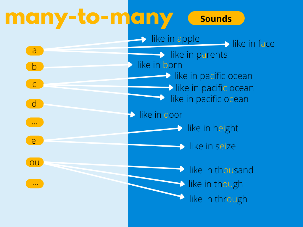
To minimize the number of mappings between characters and sounds, we should normalize our dataset. After this step, it should contain only the words and punctuation we need to verbalize digits and abbreviations, write numbers with words and expand abbreviations into their full forms.
| Raw | Normalized |
| David Bowie was born on 8 Jan 1947. | David Bowie was born on eighth January nineteen forty-seven. |
| Bakery is on 47 Old Brompton Rd. | Bakery is on forty-seven Old Brompton Road |
Moreover, we need to take care of borrowings, words from other languages, which may appear in our texts. Borrowings should be written as you hear them.
| Raw | Normalized |
| She yelled – Garçon! | She yelled – Garsawn! |
| Causal greeting in Polish is “cześć”. | Casual greeting in Polish is “cheshch”. |
Of course, you can restrain from doing that if you don’t have any borrowings in your dataset or if you enforce a specific way of reading on speakers, but for their comfort and simplicity, it is better to just write borrowings as you hear them.
Another problematic part of language normalization is acronyms. In our dataset, we decided that acronyms that are read as letters will be split with ‘-’.
| Raw | Normalized |
| UK | UK |
| OPEC | OPEC |
As in the example above, OPEC is read as a word, not as letters, therefore we don’t need to split it. The last tip on normalization is to choose a symbol set. That allows us to filter out unwanted symbols, as it will make the further stages of processing easier and simpler.
After text collecting and processing, it’s time to record and form our brand-new dataset.
Share
Authors: Marcin Walkowski, Konrad Nowosadko, Patryk Neubauer
Next in the series: How to prepare a dataset for neural Text-To-Speech — Part 2: Recordings & Audio Processing
Share

Our NLP Team at Voicelab in cooperation with the University of Lodz prepared one of the challenges at Poleval 2021.
PolEval is a set of annual ML challenges for Polish NLP, inspired by SemEval. Submissions compete against one another within certain tasks selected by organizers, using available data, and are evaluated according to pre-established procedures.
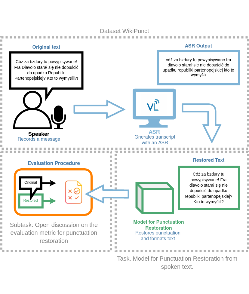
The purpose of our Task 1: Punctuation restoration from read text is to restore punctuation in the ASR recognition of texts read out loud. Along with the Task we shared the dataset and WikiPunct, consisting of over 1500 recordings and 32,000 texts. WikiPunct is a crowdsourced text and audio data set of Polish Wikipedia pages read aloud by Polish lectors. The dataset is divided into two parts: conversational (WikiTalks) and information (WikiNews). Over a hundred people were involved in the production of the audio component. The total length of audio data reaches almost thirty-six hours, including the test set. Steps were taken to balance the male-to-female ratio.
Read more about the data and the task here. Data has been published in the following repository (repository). Gold-standard test data annotation has been published in the „secret” branch.
Come and see us on 25th October at the NLP day conference on the PolEval track. First, we will introduce our Task, and the four first winners will describe their approaches.
As an official Partner, we invite you to register for the AI & NLP conference with our unique promo code: FREE524, which will give you free access to all presentations during the first two days of the conference.
Share