

Natural Language Processing
Generating paraphrases
Generating paraphrases

TRURL brings additional support for specialized analytical tasks:
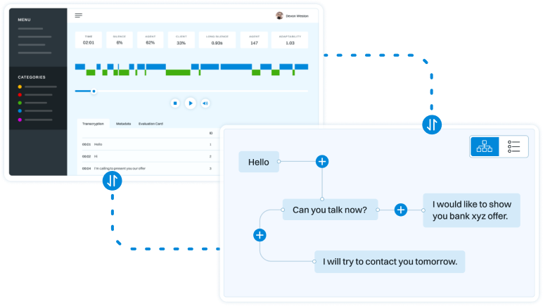
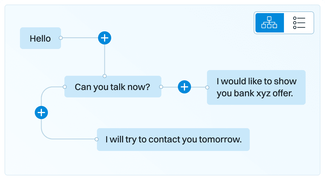
Dialog structure aggregation
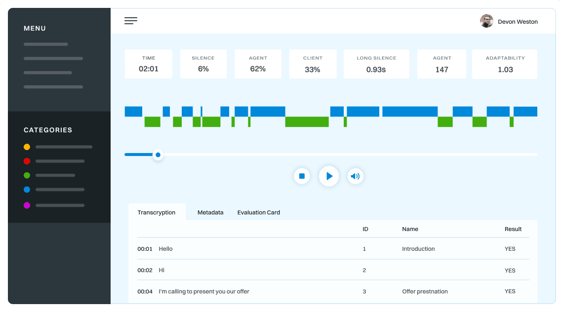
Customer support quality control
Sales intelligence and assistance
TRURL can also be implemented effectively on-premise:
We will build a GPT model for you
Trained securely on your infrastructure
Trained on your dataset

Share
A way to grasp what your NLP model is trying to communicate.
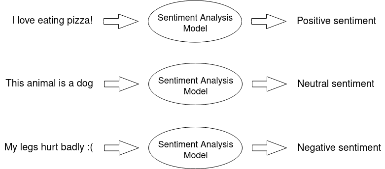
Sentiment Analysis is basically a recognition of an utterance’s emotional tone – in our case, the AI solution tells us whether given statement is negative, neutral or positive:
We have already described our approach, data used, processing of data and model architecture in more detail in a previous article. In short, we use a solution based on HerBERT and train it using labeled Twitter data.
We have decided to make use of XAI (explainable AI) in order to better understand our model’s decision-making. We wanted to see which features influence the final verdict the most and whether we can identify some room for improvement.
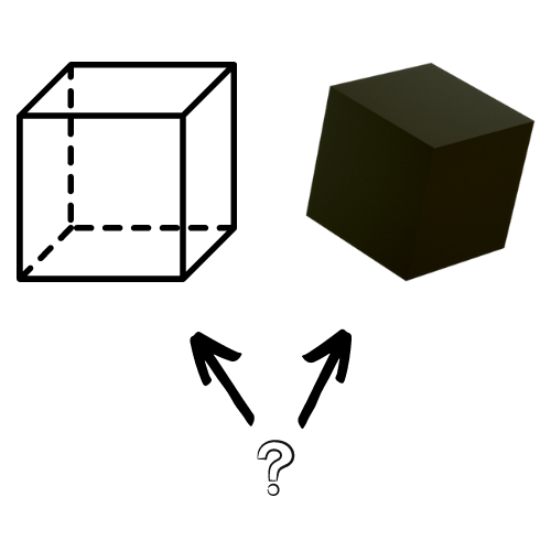
XAI (eXplainable AI) is an AI concept that enables us, humans, to understand predicted results better. We open the black box, you could say.

Most of us have heard of the term ‘black box’ when referring to Deep learning models. It is defined as a complex system or device whose internal workings are hidden or not readily understood. It has originated from the fact that usually even model developers cannot state why the AI has come to a specific conclusion.
On the one hand, some might say it is beneficial to develop deep, multilayered models without needing to understand the whole decision process, and they are not wrong. It takes away worries and makes the process somewhat convenient. However, how can we be so sure that our prediction is based on good premises?
Even if we achieve high accuracy scores on the test set, it might not be the real-world inference accuracy. The results will also be biased if the dataset is biased, and high-performance results mislead us to believe that the system is just fine. Models’ robustness is especially important in domains like medicine, finance, or law, where it is crucial to understand the reasoning behind a decision when its consequence might be fatal.
It can be highly beneficial to try and dig deeper into the unknown of mentioned above ‘black box’. The inability to fully explain AI decision-making has been quite troublesome over the years.
There is a phenomenon that can, in short, be described as Algorithm aversion – a situation where people lack trust in algorithmic model decisions, even knowing that it outperforms human beings.
People fear what they do not understand, and this is usually the case with the black box models. The inability to grasp why the AI model has decided one thing instead of another causes insecurity and doubts. In turn, that leads to a lack of trust and decision rejection that could be better than our judgment.
It is logical to assume that people would be more likely to listen to AI if they better understood the decision-making process.
We can distinguish two main types of approaches to explaining the model predictions:

building a simpler, transparent model
sing a black-box model and explaining it afterwards
Transparent ML models, such as a simpler decision tree, Bayesian models or linear regression, even though easily interpretable, have often proven to be outperformed by their black-box friends. Therefore, since we want the best performance possible, we need the additional post-hoc layer on top of our solution.
Post-Hoc meaning after the event, in our case, means an explanation done after making a prediction (or series of predictions).
Explanations can be Model Agnostic (works with any model) or Model Specific. The one that interests us the most is the Model Agnostic since it will explain any model, regardless of the architecture.
We also want to focus on the idea of the Feature Importance – to measure how an individual feature (input variable) contributes to the predicted output.
Such an approach very neatly suits the Natural Language Processing (NLP) domain.
In NLP classification problems, we are often supposed to analyze a sequence of words provided as an input and get the probability of each class affiliation as an output.
Basically, when explaining a single prediction, we want to measure how each element of an input contributes to each class probability. It’s pretty straightforward. The difficulty now is how to do it.
Over the past years, many algorithms have been developed. Here, we chose two Explainers based on their simplicity and understandability: LIME and SHAP. The solutions we use are rather intuitive and easy to grasp.
LIME is one of the first perturbation-based approaches to explaining a single prediction. As we can read on projects github page:
Lime can explain any black-box classifier with two or more classes. All we require is that the classifier implements a function that takes in raw text or a NumPy array and outputs a probability for each class.
As a result, we can apply LIME to any model that takes in raw text or a NumPy array and provides a probability for each class as an output.
But what does it do exactly?
The main idea is that it is easier to approximate the whole model with a simpler local model. How can that be achieved?
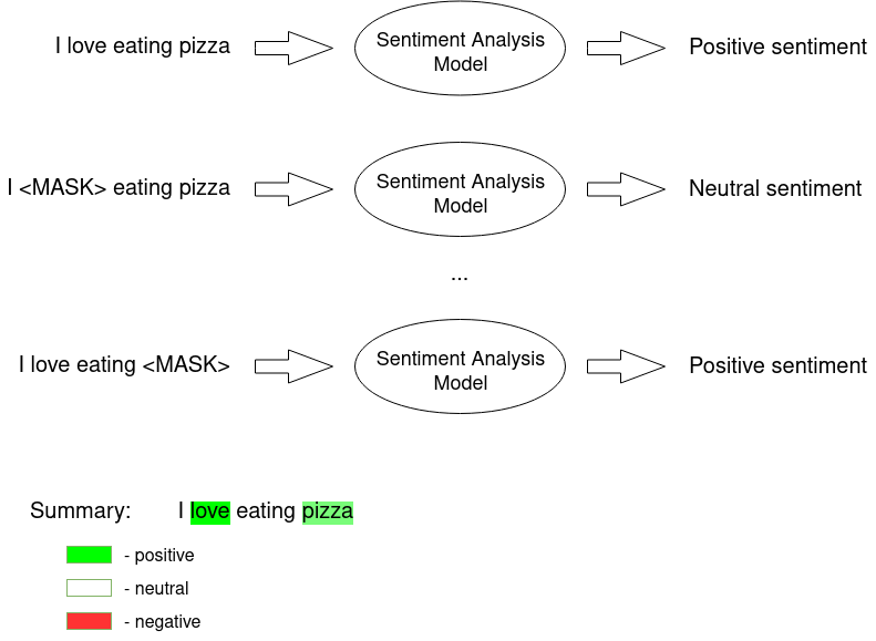
We perform a perturbation of the input sequence (e.g. we hide one sentence word (marked with MASK token)) and check how the predictions differ. Then the perturbed outputs are weighted by their similarity to the explained example.
Intuitively, an explanation is a local linear approximation of the model’s behavior. While the model may be very complex globally, it is easier to approximate it around the vicinity of a particular instance. While treating the model as a black box, we perturb the sample we want to explain and learn a sparse linear model around it as an explanation. The figure below illustrates the intuition for this procedure. The model’s decision function is represented by the blue/pink background and is clearly nonlinear. The bright red cross is the instance being explained (let’s call it X). We sample instances around X and weigh them according to their proximity to X (weight here is indicated by size). We then learn a linear model (dashed line) that approximates the model well in the vicinity of X, but not necessarily globally.
Since the input is in the form of understandable words, we can then easily interpret the provided results. On the output, we receive a list of all features and their contribution to each of the classes.
Exemplary visualisation:
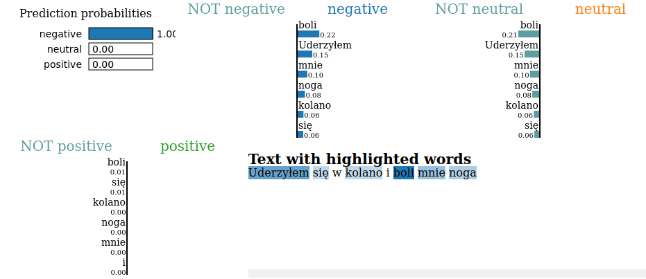
We can see in the image above how different features (words) contributed to each class. E.g. ‘boli’ caused the probability of the ‘negative’ class to rise and lowered the likelihood of the ‘neutral’ class.
This algorithm is somewhat similar to the LIME as it also perturbs input to make explanation. However, in a bit different way.
If you would like to understand all the details behind SHAP methodology, here is a great article that talks about the subject in a really understandable manner.
In short, SHAP is a calculating contribution that each feature brings to the model prediction. The contribution is based on the idea that in order to determine the importance of a single feature, all possible combinations of features should be considered (a power set in maths). Therefore, SHAP approximates all the possible models from the provided dataset (i.e., the input we have provided in a given explanation). Having all possible combinations, all of the marginal contributions are taken into account for each feature.
Marginal contribution of a certain feature is a situation where there are two almost exactly the same scenarios with the only difference being a presence (or absence) of our feature of interest.
All the marginal contributions are then aggregated through a weighted average, and the outcome represents contribution of a given feature to a given class. The summary can then be visualised, e.g. with a force plot, such as the one below:
Here, the features that increase the probability for a given class are highlighted with red and those that lower it with blue. The base value is the average model output over the training dataset we have passed.
Having our algorithms selected and explained, we can see how they perform in practice. In our case, during the analysis of Polish utterance emotional tone.
To recap, we are using model based on HerBERT (Polish BERT), and we have distinguished three classes – negative, neutral, and positive.
Exemplary utterance to analyse:
Jutro pierwszy dzień w mojej nowej pracy. Cieszyłabym się, ale jestem bardzo zestresowana i spięta
True sentiment: negative
Predicted sentiment: negative
As we can see, the model has correctly predicted negative sentiment within the provided sentence, even though the example is a little tricky. Now, let’s move on to the explaining process and check which features influenced this decision.
Firstly, let LIME show its performance. We load our model from a checkpoint:
device = 'cpu'
        model = HerbertSentiment.load_from_checkpoint(model_path,
                                                        test_dataloader = None,
                                                        output_size = 3,
                                                        hidden_dim = 1024,
                                                        n_layers = 2,
                                                        bidirectional = True,
                                                        dropout = 0.5,
                                                        herbert_training = True,
                                                        lr = 1e-5,
                                                        training_step_size = 2,
                                                        gamma = 0.9,
                                                        device = device,
                                                        logger = None,
                                                        explaining = True)
Then we setup the LIME:
tokenizer_path = "allegro/herbert-base-cased"
        tokenizer = AutoTokenizer.from_pretrained(tokenizer_path)
        target_names = ['negative', 'neutral', 'positive']

        explainer = LimeTextExplainer(class_names=['negative', 'neutral', 'positive'])
Finally, we make the explanation.
input = "Jutro pierwszy dzień w mojej nowej pracy. Cieszyłabym się, ale jestem bardzo zestresowana i spięta"

        explanation = explainer.explain_instance(input, model.forward, num_features=6, labels=[0,1,2])
… and print the results:
print ('Explanation for class %s' % target_names[0])
        print ('\n'.join(map(str, exp.as_list(label=0))))
        print()
        print ('Explanation for class %s' % target_names[1])
        print ('\n'.join(map(str, exp.as_list(label=1))))
        print()
        print ('Explanation for class %s' % target_names[2])
        print ('\n'.join(map(str, exp.as_list(label=2))))
Those messy numbers in the picture define how a certain word influenced each of the classes. If a number is >0 then it increased the chance for the class. On the contrary, if it is <0 it decreased it.
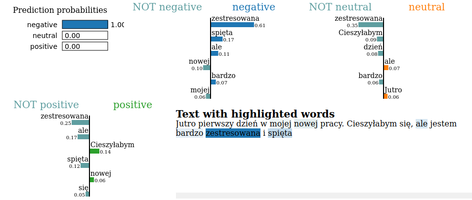
explanation.show_in_notebook()
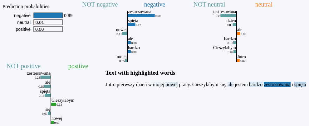
In the dedicated LIME visualisation above, it is a bit easier to interpret the results. We can quickly tell which tokens were the most influential for which class. For example, the word ‘zestresowana’ significantly impacted all categories, greatly increasing the chance for negative and reduces bothneutral and positive ones.
As you can see, it can provide some helpful insight.
Now, let’s compare all this to SHAP…
We load the model in the same manner:
device = 'cpu'
        model = HerbertSentiment.load_from_checkpoint(model_path,
                                                        test_dataloader = None,
                                                        output_size = 3,
                                                        hidden_dim = 1024,
                                                        n_layers = 2,
                                                        bidirectional = True,
                                                        dropout = 0.5,
                                                        herbert_training = True,
                                                        lr = 1e-5,
                                                        training_step_size = 2,
                                                        gamma = 0.9,
                                                        device = device,
                                                        logger = None,
                                                        explaining = True)
Then we set up the SHAP:
tokenizer_path = "allegro/herbert-base-cased"
        tokenizer = AutoTokenizer.from_pretrained(tokenizer_path)
        target_names = ['negative', 'neutral', 'positive']

        explainer = shap.Explainer(model, tokenizer)
Prepare methods for the results visualization:
def print_explanation(shap_values):
            values = shap_values.values
            data = shap_values.data
            for word, shap_value in zip(data[0], values[0]):
                print(word, shap_value, '---', target_names[np.argmax(shap_value)])

        def print_contribution(shap_values):
            print('\n')
            print("Contribution to negative class")
            shap.plots.text(shap_values[0, :, 0])
            print('\n')
            print("Contribution to neutral class")
            shap.plots.text(shap_values[0, :, 1])
            print('\n')
            print("Contribution to positive class")
            shap.plots.text(shap_values[0, :, 2])
Finally, we make the explanation…
input_to_explain = ["Jutro pierwszy dzień w mojej nowej pracy. Cieszyłabym się, ale jestem bardzo zestresowana i spięta"]

        shap_values = explainer(input_to_explain)
… and print the results:
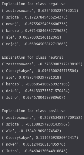
print_explanation(shap_values)
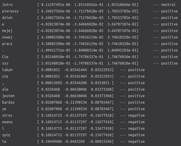
We can see numbers that show how sentence tokens contribute to each class, much like they do in LIME. Additionally, there is a dominating sentiment shown on the right.
You can notice that some words are divided and analyzed strangely since SHAP is using the HerBERT tokenizer for the explanation process. The tokenizer analyses the input sequence and looks for each of the tokens (words) in its dictionary. If a particular word does not exist there, it is divided into parts that do. E.g. ‘Uwielbiam’ will be divided into ‘Uwielbi’ and ‘am’. This process helps to ignore possible flection noise resulting from Polish grammar rules (a male variant of a word will differ from a female variant of the same word).
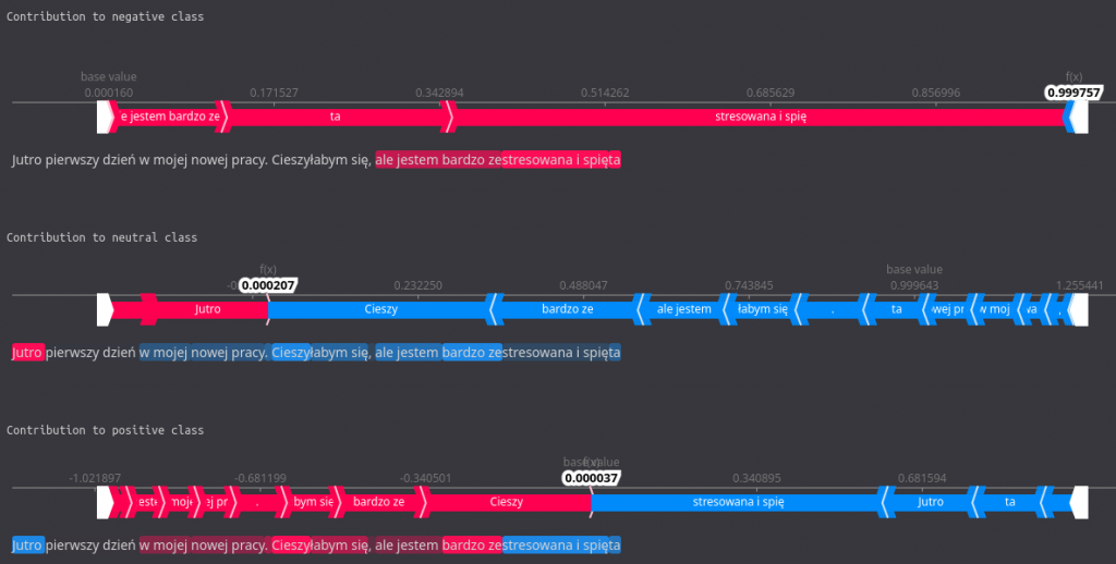
print_contribution(shap_values)

In this more colorful visualization, the same data is presented but in a more comprehensible manner. There is a force plot for each of the classes, along with all of the words contributing. Those marked with red color increased probability for a given class, and those in blue decreased it. We can easily see which tokens were the most influential, both on the force plot and in the highlights in the sentence below the plot.
For instance, we observe that the words (or their parts) ’zestresowana i spięta’ influence the negative sentiment quite a bit while lowering the positive one significantly.
Proper interpretation of such visualisations can give us a good idea of how our model thinks and influences the result the most.
As you can see, XAI provides us with some interesting and valuable insight into our model. The explanation process is not as complex as it might seem, and it is worth the burden considering the benefits. Proper interpretation of the results, including the understandable visualizations, can give us a good idea of how our model ‘thinks’ and what influences the predictions the most.
If your machine learning problem regards one of the domains where algorithm trust is crucial to be developed and where algorithm aversion might cause you a headache, explainable AI comes to the rescue. Keep this in mind the next time you want to dig deeper into your algorithm.
Share
Authors: Filip Żarnecki, Michał Laskowski